
In my previous note, Introduction to Data Structures and Algorithms - DSA #1, I introduced several key concepts of data structures and algorithms. In this note, we'll dive into analyzing algorithm efficiency by exploring the algorithm complexity, the order of growth, and asymptotic notations!
Introduction to Algorithm Analysis
Let's talk about something that keeps computer scientists up at night - algorithm efficiency!
Next time you're scrolling through your social media feed and everything loads instantly, remember that powerful and efficient algorithms are working their magic behind the scenes!
So how do computer scientists actually measure how efficient an algorithm is?

Algorithm Analysis
In today’s computers, the speed and memory are two primary important considerations from a practical point of view. "Analysis of algorithms" refers to evaluating an algorithm's efficiency in terms of two key resources—running time and memory space.
There are two kinds of efficiency:
- Time efficiency indicates how fast an algorithm runs.
- Space efficiency refers to the amount of memory required by an algorithm.
Wait... while time efficiency concerns are clear, is space efficiency still relevant today?
Let’s consider this simple problem: “Given the array consists of integers. Rearrange the array such that all odd numbers appear on the left, sorted in ascending order, and all even numbers appear on the right, sorted in descending order.“
There are various solutions to this problem. Here are the two most common approaches:
- One solution is to create two new arrays, and . We iterate through array , placing odd numbers in and even numbers in . After sorting both arrays, we combine them back to the array .
A[1...n] // The original array consists of n integers

// We need to declare two new arrays of size n
B[1...n] // Consists of only odd numbers
C[1...n] // Consists of only even numbers

// Let's calculate the memory cost of this solution.
// An integer variable in the memory usually takes 4 bytes.
//    + The memory cost of an array: 4 * n (bytes)
//    + The memory cost of 3 arrays: 3 * 4 * n (bytes)
// Total cost: 3 * 4 * n (bytes)- Another solution is to do all of the sorting operations on the original array .
A[1...n] // The original array consists of n integers

// Since all operations are performed on the original array,
// we don't need to declare new ones, so the memory cost of
// this solution remains 4 * n (bytes)
In the past, programmers strongly preferred the second solution due to the high cost of memory—for example $300 per megabyte in 1986 compared to just $0.005 in 2024. See for yourself, a mere 2MB of RAM cost about $600 back then, while today you can get an 8GB RAM stick for around $40. Back then, developers had to optimize their programs to use minimal memory, a constraint that rarely concerns us today.
Though memory efficiency still matters somewhat since memory allocation affects performance, this note will focus primarily on time complexity.
Measuring an Input’s Size
It is understandable that almost all algorithms run longer on larger inputs. When we deep dive into investigating an algorithm’s efficiency, the major work that goes into this is to construct a function of some parameter indicating the algorithm’s input size.
It is worth noting that the value of must be large enough. Algorithms often reveal their true efficiency only with larger inputs, as small inputs may not showcase their strengths. This raises the question: “How large is large enough?”
The answer depends on the specific problem the algorithm aims to solve. Consider a simple example of multiplying two numbers with digits:
- The oldest and simplest method—long multiplication—involves multiplying every digit in the first number by every digit in the second and adding the results.
- The Karatsuba multiplication method breaks the problem into smaller parts, performs multiplication on those parts, and combines the results.
Mathematically, the complexity of the long multiplication method is , while the Karatsuba method is only . If you don't understand the reason behind this, don't worry! Since the exponent is larger than , the Karatsuba method should be more efficient, right?
Actually, this isn't true with smaller inputs. The Karatsuba multiplication method only begins to outperform its traditional counterpart when . When is smaller than , the overhead of splitting and combining makes this method less efficient.
However, “large enough” doesn't mean using excessively large inputs. For example, feeding 64 discs at a rate of 1 disc per second into the algorithm that solves the Tower of Hanoi puzzle would be too large for this algorithm to handle (which would take 584 billion years to solve)!
In most cases, selecting such a parameter is quite straightforward.
Units for Measuring Running Time
Let's say there are two programmers, each tasked with writing a computer program to solve the same problem. Their processes are demonstrated in the flowcharts below:
How do we measure the performance of each programmer's algorithm? At first glance, it seems straightforward—just measure the runtime in seconds, milliseconds, or even nanoseconds if you’re feeling fancy! Programmer A's implementation took 1 hour to produce the output, while Programmer B's took 3 hours. But can we really conclude that Programmer B's algorithm is less effective based on these times alone?
Here’s the catch: relying on raw execution time has some serious drawbacks:
The language used in writing the program
Imagine you have two programs, one written in Python and the other in C++, both implementing the same sorting algorithm. Due to C++ being a compiled language while Python is an interpreted one, the C++ program is likely to run faster, even though the underlying algorithm is the same.
The programmer’s skill
Consider two programmers tasked with implementing an algorithm. Beginners often write brute-force solutions that are slow but easy to understand, experienced programmers typically implement cleverer and more optimized approaches that run faster.
Additionally, I'd like to give some examples to point out that even small differences in programming techniques can significantly impact performance on the same program:
- When declaring an array, declaring the element type as
intcan make the program run faster than declaring asdouble. This is because the latter requires processing floating-point number, which is more computationally intensive. - Identifying duplicated expressions and replacing them with a single variable holding the computed value can also helps improve the speed of the program.
The speed of a particular computer
If you run the same program on a high-end gaming PC and a budget laptop, the difference in processing power and hardware will significantly impact the execution time. The algorithm's efficiency remains constant, but the hardware influences the observed performance.
It is also of note that even with the same processor, the performance might differ. For example, on the Cortex-M7 chip, it has an optional floating-point unit (FPU) for processing floating-point numbers. In programs that require processing these numbers, silicons which are designed with the FPU can perform the operation at the hardware level, while those without the FPU relies on software-emulated implementations which is much slower and inefficient.
The compiler used in generating the machine code
Compilers convert your code into machine-readable instructions, and different compilers (like GCC vs. Clang) can optimize code differently. In addition, optimization flags can yield varying performance results for identical code.
The test set
When designing an algorithm, there’s a question that comes to mind: “Does the program or the algorithm work correctly for any valid input data?”. To answer that question, programmers have to build a test set.
Let’s say you’re testing a sorting algorithm. Using a small, sorted dataset to test a sorting algorithm might give the illusion of exceptional performance. However, the algorithm's true efficiency would be revealed when tested on a large, unsorted dataset.
...and even more! This is why we need a metric that remains independent of these factors in order to measure an algorithm’s efficiency.
Therefore, one possible approach is to find the function which counts how many times each operation in the algorithm executes. Let’s take a look at some examples:
Example 1: Finding the largest element in an array
max = a[1]; // 1 operation

for (i = 2; i <= n; i++) {
  // i = 2: 1 operation
  // i <= n: n - 1 operations
  // i++: n - 1 operations

  if (a[i] > max) { // n - 1 operations
    max = a[i]; // t operations, 0 ≤ t ≤ n - 1
  }
}

return max; // 1 operationExample 2: Sorting an array in ascending order
for (i = 1; i < n; i++) {
  // i = 1: 1 operation
  // i < n: n - 1 operations
  // i++: n - 1 operations

  for (j = i + 1; j <= n; j++)
  // j = i + 1: n - 1 operations
  // j <= n: (n(n - 1)) / 2 operations
  // j++: (n(n - 1)) / 2 operations

    if (a[i] > a[j]) { // (n(n - 1)) / 2 operations
      t = a[i];     //
      a[i] = a[j];  // t operations, 0 ≤ t ≤ (n(n - 1)) / 2
      a[j] = t;     //
    }
}Example 3: Multiplying two matrices
for (i = 1; i <= n; i++) {
  // i = 1: 1 operation
  // i <= n: n operations
  // i++: n operations

  for (j = 1; j <= n; j++) {
    // j = 1: n operations
    // j <= n: n^2 operations
    // j++: n^2 operations

    c[i][j] = ø; // n^2 operations

    for (k = 1; k <= n; k++) {
      // k = 1: n^2 operations
      // k <= n: n^3 operations
      // k++: n^3 operations

      c[i][j] = c[i][j] + a[i][k] * b[k][j]; // n^3 operations
    }
  }
}Based on the examples above, counting individual operations proves both overly complex and typically unnecessary. Thus, the solution is to…
- identify the operation contributing the most to the total running time.
- compute the number of times this operation is executed.
Such an operation is called the basic operation.
The Basic Operation
In computer science, the definition of the basic operation doesn’t exist. Instead, people just informally describe it.
The basic operation can be described as:
- It is usually the most time-consuming operation.
- It is usually in the algorithm’s innermost loop.
- It usually relates to the data that needs to be processed.
Therefore, the time efficiency of an algorithm is measured by counting the number of times the algorithm’s basic operation is executed, on inputs of size .
Let's revisit the above examples, find the basic operation, and construct the function that represent the number of times the basic operation executes:
Example 1: Finding the largest element in an array
max = a[1];
for (i = 2; i <= n; i++) {
  if (a[i] > max) { // --> This is the basic operation
    max = a[i]; // --> This is not the basic operation,
                //     because it only get executed at
                //     most t times (t ≤ n - 1) -> does
                //     not significantly contribute to
                //     the overall runtime.
  }
}
return max;Example 2: Sorting an array in ascending order
for (i = 1; i < n; i++) {
  for (j = i + 1; j <= n; j++)
    if (a[i] > a[j]) { // --> This is the basic operation
                   // --> These are not basic operations,
      t = a[i];    //     because they only get executed
      a[i] = a[j]; //     at most t times (t ≤ (n(n-1))/2)
      a[j] = t;    //     -> don't significantly contribute
                   //     to the overall runtime.
    }
}Example 3: Multiplying two matrices
for (i = 1; i <= n; i++) {
  for (j = 1; j <= n; j++) {
    c[i][j] = ø;
    for (k = 1; k <= n; k++) {
      c[i][j] = c[i][j] + a[i][k] * b[k][j]; // --> This is the basic operation
    }
  }
} Some might argue that the operation c[i][j] = c[i][j] + a[i][k] * b[k][j] could be split into three separate basic operations: addition +, multiplication *, and assignment =, with . However, since this is a compound statement, treating it as a single basic operation is equally valid in this field.
Let's have a look at another interesting example:
i = 1;
while ((i <= n) && (a[i] != k))
  i++;
return i <= n;
In this example, identifying the basic operation can be a little bit tricky. While all operations are essential for the algorithm to function, we need to determine which operation contributes most significantly to the running time.
Many would assume that both and are basic operations. However, this isn't quite right. In this algorithm, alone serves as the basic operation! Let’s simplify the code further by using a sentinel to eliminate the above end-of-array solution:
a[n + 1] = k; // sentinel
i = 1;
while (a[i] != k)
  i++;
return i <= n;
You may start to see why is the basic operation!
As a side note, in the code without the sentinel above, the computer must perform two checks: and . With the sentinel, you only need one extra block of memory, and the program runs faster by removing the overhead condition in each iteration of the loop!
The Order of Growth
Order of Growth of the Running Time
Consider two different algorithms designed to solve the same problem. Let and represent the number of times each algorithm executes its basic operation.
As shown in the table, for large values of , the lower-order terms become negligible. Therefore, only the leading term of a polynomial is considered. This is called the order of growth of the running time. We also ignore the leading term's constant coefficient since it has less impact on computational efficiency than the order of growth when dealing with large inputs.
Let’s use the function of the basic operation from Example 2 above:
By removing both the constant coefficient of the leading term and any lower-order terms, we can determine the order of growth:
The Typical Growth Rates
Think of growth rates as the speedometer of your algorithms, how their runtime scales with the size of the input. The bigger the input, the longer it takes, but the rate of increase varies based on the growth rates.
Let’s look at some of the most typical growth rates:
| Function | Name | Description |
|---|---|---|
| Constant time | The runtime is constant and does not depend on the input size. Examples: - Search operation on hash tables (approaches constant time) - Accessing an element array using its index | |
| Logarithmic time | The runtime increases slowly as the input size increases. Examples: - Binary search | |
| Linear time | The runtime increases proportionally to the input size. Examples: - Linear search in an array - Calculate the sum of every element in an array | |
| Linearithmic or Quasilinear time | Examples: - Some sorting algorithms, such as merge sort, etc. | |
| Polynomial time | The runtime grows polynomially with the input size. The most common values of are and . Examples: - Some sorting algorithms, such as bubble sort, etc. - Multiplying 2 matrices | |
| Exponential time | The runtime skyrockets as the input size grows. The most common value of is . Examples: - Tower of Hanoi puzzle - Calculating the element of the Fibonacci sequence using divide and conquer | |
| Factorial time | The runtime explodes as the input increases. Examples: - Generating all permutations of a set |
Worse-case, Best-case, and Average-case
We know that the efficiency of many algorithms depends on the size of the input. However, another contributing factor is the distribution of a particular input.
Thus, the complexity of such algorithm needs to be investigated in three cases:
- The worse-case running time
- The best-case running time
- The average-case running time
Consider the linear search algorithm on the following array:
Worse-case running time
If we search for the value , we must iterate through every item in the array, resulting in the longest running time.
In other words, the worse-case complexity is an upper bound on the running time for any input. Typically, we analyze algorithms by examining the worse-case scenario, as it ensures that the algorithm will never take any longer.
Best-case running time
What if we search for the value ? Surely, we only need to do one comparison at the first element of the array. It just takes the shortest time to complete the algorithm!
Best-case complexity is a lower bound on the running time for any input, which also indicates the fastest running time. Analyzing the best-case is almost impractical, because guaranteeing a lower bound on the algorithm doesn’t offer much insight; the algorithm could still take a very long time to run!
Average-case running time
This is a little bit tricky.
The average-case complexity is an estimation of the average running time for every possible inputs. This type of analysis is infrequently performed because it is often challenging and significantly more complex than analyzing worst-case and best-case scenarios. It cannot be calculated simply by averaging the worst-case and best-case complexities. Instead, we must know the probability of different input arrangements.
In the example above, we only know the average number of comparisons needed in the array would be .
Asymptotic Notations
The order of growth of an algorithm is regarded as the primary indicator of the algorithm’s efficiency. To compare and rank such orders of growth, computer scientists use three notations:
- Big O Notation ()
- Big Omega Notation ()
- Big Theta Notation ()
Think of these notations as powerful tools that allow us to compare and rank the growth rates of different algorithms, helping us make informed decisions about which algorithm is best suited for a particular task.
In the following discussions, and can be any non-negative functions defined on . If denotes the running time of an algorithm, then denotes some simple function to compare with . For simplicity, let .
Big O Notation
is the set of all functions with a lower or same order of growth as . This notation provides an upper bound on the growth rate of a function and describes the worst-case scenario for an algorithm's runtime.
For example, if an algorithm's runtime is , it means that the runtime will never grow faster than polynomially with the input size.
Big Omega Notation
is the set of all functions with a higher or same order of growth as . This notation provides an lower bound on the growth rate of a function and describes the best-case scenario for an algorithm's runtime.
If an algorithm's runtime is , it means that the runtime will never grow slower than polynomially with the input size.
Big Theta Notation
is the set of all functions with the same order of growth as . This notation provides both an upper and lower bound on the growth rate of a function, which means that the growth rate of the function is exactly the same as the function it's being compared to. Obviously, is a much stronger statement than and .
If an algorithm's runtime is , it means that the runtime will grow polynomially with the input size, both in the best-case and worst-case scenarios.
Big Theta () is the most informative of the three notations because it provides a tight bound on the growth rate. However, Big O () is often used in practice because it's easier to determine and often provides sufficient information for comparing algorithms.
Understanding asymptotic notations is crucial for analyzing and comparing algorithms effectively. By using these notations, we can determine which algorithm will perform best for a given input size and make informed choices when designing and implementing programs.
Additional Notes
Execution Time of Basic Operators
There are 4 common arithmetic operators: addition, subtraction, multiplication, and division. The difference in execution time of these operations are pretty obvious.
Arithmetic Operators
- Addition/subtraction: These are simple and straightforward operations at the hardware level, meaning they’re able to run very fast.
- Multiplication: This operation involves multiple additions and shifts, therefore it is more complex and runs slower than addition and subtraction.
- Division: This is the slowest arithmetic operation, because it requires iterative process of subtraction and shifting, and even with additional floating-point number processing!
But what about comparison and assignment operators? Which is faster than the other?
Let’s see how each operator works under the hood!
In order to compare the speed of these two operators, we need to first explore the CPU registers. Located in the computer processor, the registers are the fastest read/write memory units that store values for data processing and instruction execution.
Comparison Operator
When a comparison operation is executed, for example a < b, the instruction is passed into the CPU, while the two registers R1 and R2 store the value of a and b as the operands, respectively. The Op Code is also decoded to determine the operation type (in this case, the Op Code might represent a CMP - comparison operation).
Since the value of a and b are assigned to these two registers, the CPU can quickly read the content of the registers and determine the result of the comparison.
Assignment Operator
In a processor, the number of registers is very limited, typically ranging from 8 to 32 general-purpose registers. This creates challenges when working with large amounts of data, such as assigning a value to every element of an array with elements. Since there aren't enough registers to hold the entire array, the data must be stored in RAM.
When an assignment operation executes, the Op Code represents a MOV (move/copy operation), and registers like R1 and R2 hold either the value to be copied or the source/destination memory addresses. If the data resides in RAM, the CPU must access it, which is significantly slower than accessing registers. This reliance on slower RAM significantly impacts the operation's overall speed.
In conclusion, the comparison operator is significantly faster than the assignment operator!
How Compilers Optimize Code
A compiler is a true masterpiece of computer science. This diagram demonstrates the passes of compilers behind the scenes:
In the compiler, the Optimization Pass plays an important role in improving code quality through three key factors:
- Speed: Makes the program run faster
- Size: Reduces the program's size. This is especially important for control programs in devices like washing machines, which must fit within limited ROM memory.
- Power efficiency: Particularly valuable for programs running on mobile devices.
First, the Front-end Pass generates linear intermediate code (or 3-address code). Then in the Optimization Pass, this code is transformed into a data-flow diagram, which may look something like this:
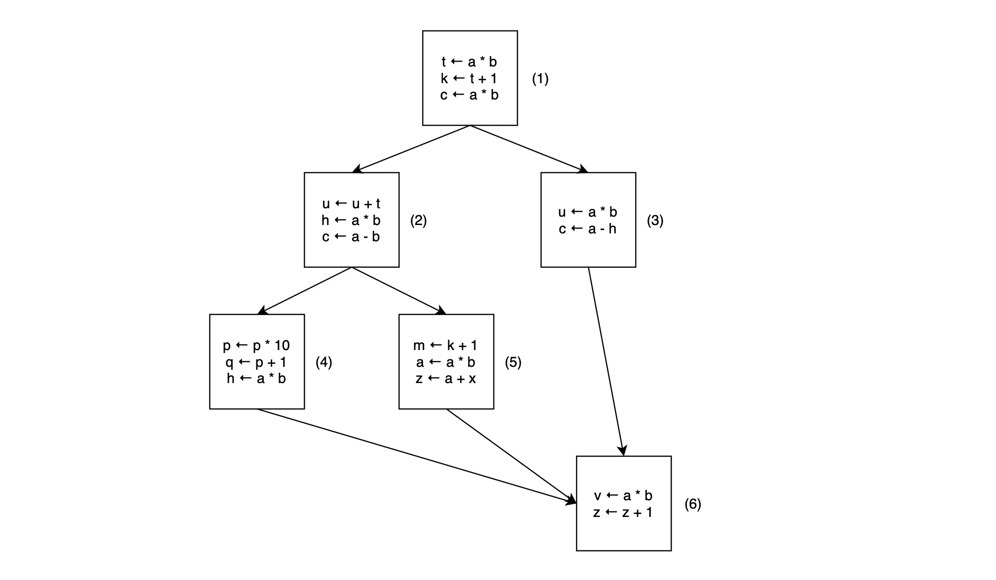
In the Optimization Pass, there are multiple modules, each designed to perform a specific optimization on the intermediate code. And one of the techniques used by the Optimization Pass is Common Subexpression Elimination, which searches for identical expressions and replaces them with a single variable holding the computed value.
In the example data-flow diagram above, the compiler defines a new variable to store the value of . It then replaces all expressions in blocks through with , reducing the number of computations needed. While humans can easily identify these replaceable expressions by examining the diagram, teaching computers to perform this task is more complex. Compiler designers must create a system of language equations to help the computer locate these expressions.
Fun fact: Free compilers may or may not include the Optimization Pass. Therefore, software companies often invest in premium compilers that maximize program optimization. With these expensive compilers utilizing heavy optimization algorithms, the compiled program can run up to 30% faster!
👏 Thanks for reading!