
Let’s deep-diving into four machine learning algorithms: K-Nearest Neighbors, K-Means Clustering, Linear Regression, and Support Vector Machine!
K-Nearest Neighbors (KNN)
Basic Concept of K-Nearest Neighbors
K-Nearest Neighbors (KNN) is one of the most popular algorithm in machine learning.
Unlike traditional machine learning methods that learn a target function, KNN doesn't build a clear model for the target function.
Instead, it memorizes the training data. When a new data point needs a prediction, KNN looks at its nearest neighbors in the training set.
The prediction process is somewhat similar to how people would assess potential partners in real life. Rather than making one-sided judgments, you might want to learn about someone’s personality by observing their family or speaking with their close friends and neighbors!
How KNN Works
The KNN algorithm includes two key components:
- A distance measurement: This determines how ‘close’ the two data points are to each other.
- : The number of nearest neighbors considered for future prediction.
Let’s consider an example classification problem:
Given the dataset consists of two classes, and . There’s a new point, , (shown as a blue dot) needs to be classified into one of these classes.
The KNN algorithm assigns a class to based on the majority class among its nearest neighbors.
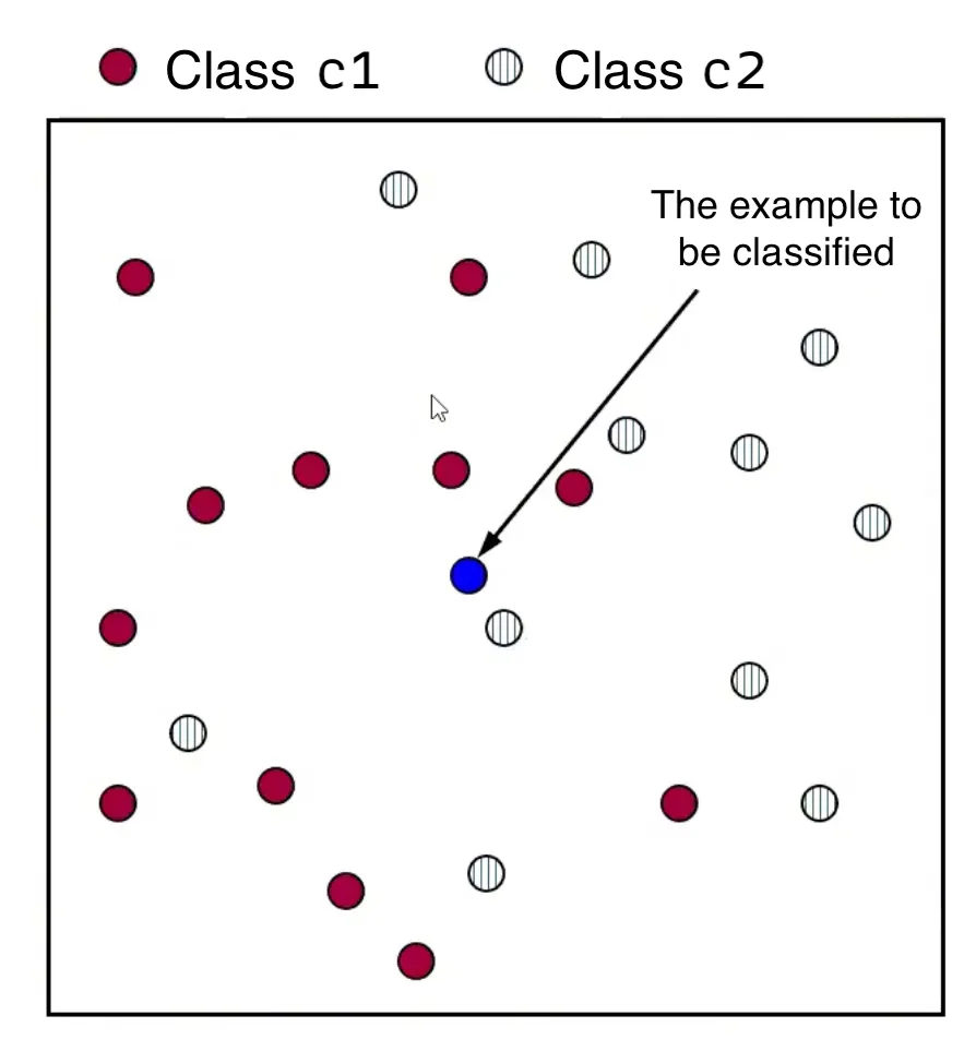
Case :
The closest neighbor to belongs to class . Therefore belongs to class .
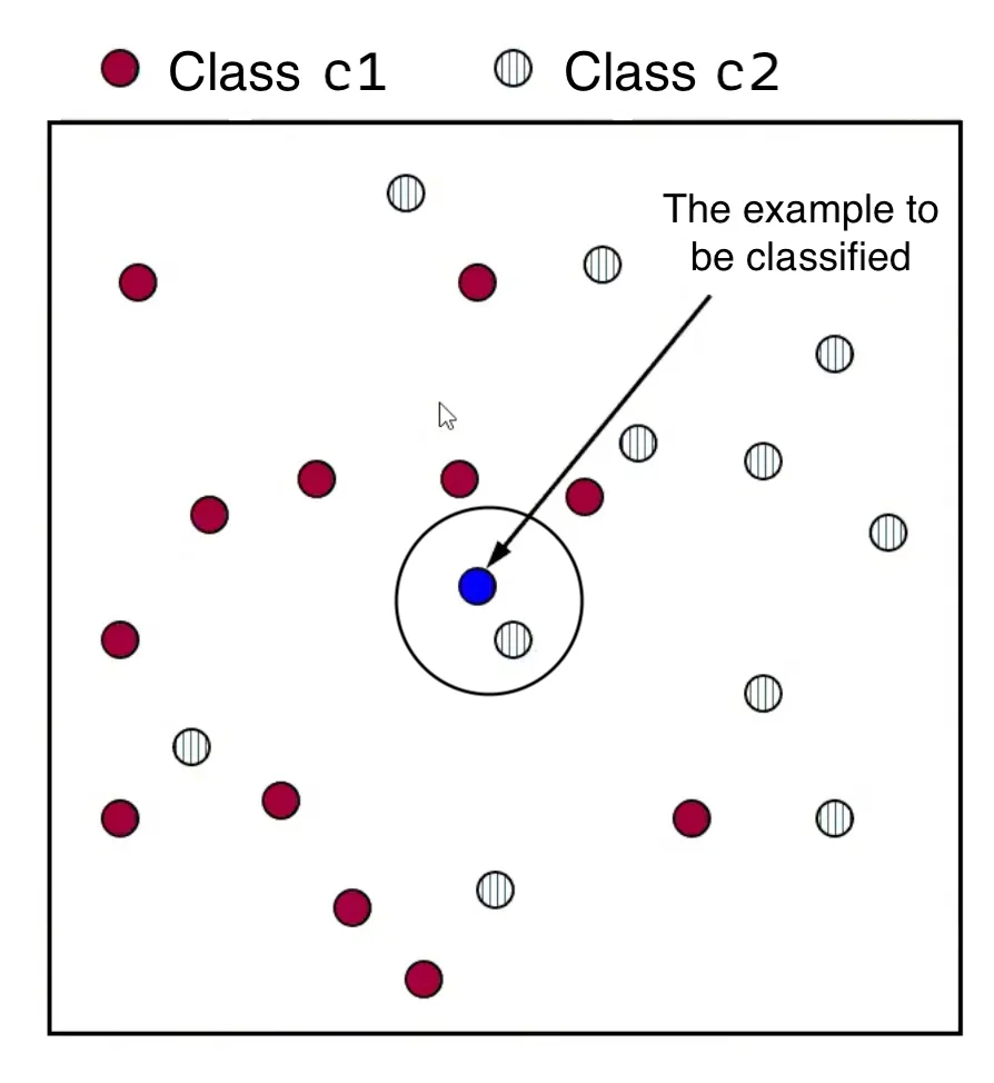
Case :
The closest neighbors to are examined. Since class has more neighbors, is assigned to class .
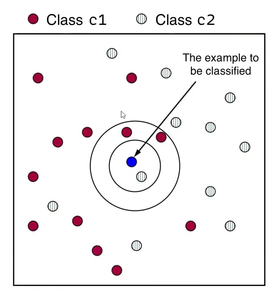
Case :
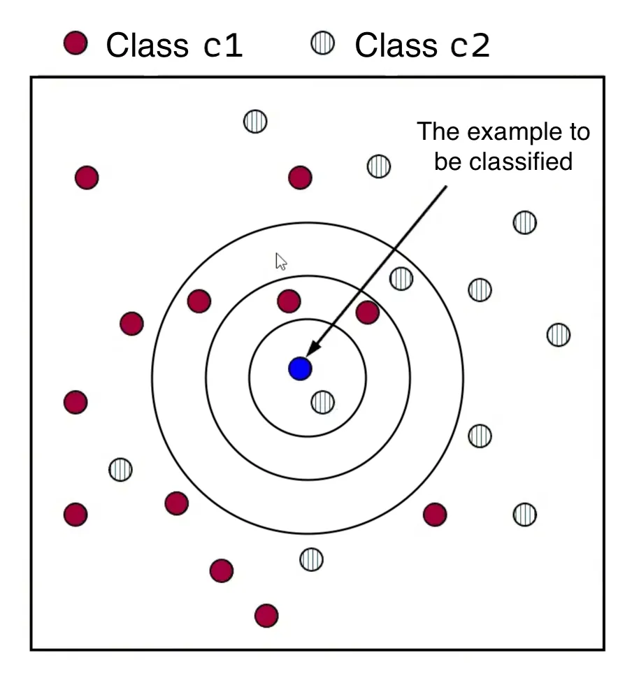
The closest neighbors to are examined. Since class has more neighbors, is assigned to class .
In Classification Problems
- For a new data point , calculate the distance between and every training data point in the dataset .
- Form a set, , consisting of the nearest neighbors of . This involves selecting the data points in that have the smallest distance to , as determined by a chosen distance function.
- Assign to the class that appears most frequently among the classes of its nearest neighbors in the set . This is known as “the majority class”.
In Regression Problems
- Similarly, we first need to calculate the distance between the new data point and each training example in the dataset .
- Identify the nearest neighbors of , forming the set .
- Predict the output value for by averaging the output values of its nearest neighbors in :
Distance Functions
Alright, so we’ve briefly mentioned the distance function in the process of solving the above problems, what exactly are those?
The distance function, often denoted as , plays an important role in the KNN method. They determine how the similarity or dissimilarity between data points is measured. The choice of distance function can significantly impact the performance of the KNN algorithm. Typically, the distance function is predetermined and remains constant throughout the learning and classification/prediction processes.
Normally, when the input attributes are real numbers (), we usually use geometric distance functions for KNN. These includes the Minkowski, the Manhattan, the Euclidean, and the Chebyshev distance functions.
- The Minkowski distance (-norm): This is a generalized distance metric. In this formula, different values of yield different distance metrics.
- The Manhattan distance (): This calculates the distance as the sum of absolute differences between the coordinates of the data points.
- The Euclidean distance (): This is the most commonly used distance function, which involves calculating the straight-line distance between two points.
- The Chebyshev distance (): This calculates the maximum absolute difference between the coordinates of the data points.
Data Normalization
Normalization the data ranges is an important step in the KNN algorithm, especially when dealing with input features that have different scales or value ranges. Without normalization, features with larger values can dominate the distance calculations, leading to skewed results.
Let’s consider a dataset with features like , (monthly), and (in meters).
- is a specific example in the dataset.
- is the value to be classified.
Let’s calculate the distance between and :
As can be seen from the calculation, values are much larger than those for or , which means the distance between two data points will be dominated by the difference in . As a result, this can overshadow the contributions of and and potentially skewing the overall result.
To address this issue, it is essential to normalize the range of input attributes so that each feature contributes more equitably to the distance calculation.
The most frequently used normalization ranges are and . For each attribute , the normalized value can be calculated as .
Let’s revisit the above example and normalize the and data points to the range:
- is normalized to .
- is normalized to .
- is normalized to .
- is normalized to .
By normalizing the features, you ensure that each feature contributes proportionally to the distance calculation, leading to more accurate and reliable KNN results.
K-Nearest Neighbors Using scikit-learn
This is a basic implementation of the KNN algorithm using the scikit-learn library:
- Declaration: This involves importing the necessary KNN classifier or regressor from the scikit-learn library.
from sklearn.metrics import precision_score, recall_score, accuracy_score from sklearn.neighbors import KNeighborsClassifier - Initialization: Create an instance of the KNN classifier or regressor, specifying parameters such as the number of neighbors (K) and the distance metric. For example, you can specify the distance metric (Euclidean, Minkowski, etc.) and the value of for the Minkowski distance.
knn_classifier = KNeighborsClassifier(n_neighbors = 10, metric = 'minkowski', p = 2, weights = 'distance') - Training: Train the KNN model using the training data. In Scikit-learn, this typically involves calling the
fit()method on the KNN object and passing the training data as arguments.knn_classifier.fit(X_train, y_train) - Prediction: Use the trained KNN model to make predictions on new, unseen data. This involves calling the
predict()method on the KNN object and passing the new data as an argument.y_pred_knn = knn_classifier.predict(X_test) print('Accuracy: ', accuracy_score(y_test, y_pred_knn)) print('Precision: ', precision_score(y_test, y_pred_knn)) print('Recall: ', recall_score(y_test, y_pred_knn))
K-Means Clustering
Basic Concept of K-Means Clustering
K-Means Clustering is a popular partition-based method used to divide a dataset into clusters. The data is represented as where each is an observation in the form of a vector in an -dimensional space.
The idea is to partition a dataset into clusters, where each cluster has a centroid (center point). The data points are assigned to the cluster with the nearest centroid.
In contrast to the K-Nearest Neighbors algorithm that works with labeled data in supervised learning problems, we often use the K-Means Clustering algorithm with unlabeled datasets in unsupervised learning problems. While the algorithm is efficient and robust, having to predefine or the number of clusters is one of its biggest limitations.
How K-Means Clustering Works
The K-Means Clustering algorithm includes two key components:
- A distance function : This determines the distance between data points and centroids.
- : The number of clusters to be created, which is predetermined.
Consider we have a dataset , the number of clusters , and a distance function :
- Step 1: Randomly select observations from the dataset to serve as initial centroids for the clusters.
- Step 2: Repeat step 2.1 and 2.2 until a convergence criterion is met.
- Step 2.1: Assign each observation to the nearest cluster based on the distance to the centroid.
- Step 2.2: Recalculate the centroid of each cluster based on the observations assigned to it. The centroid is computed by averaging the coordinates of all the points in the cluster.
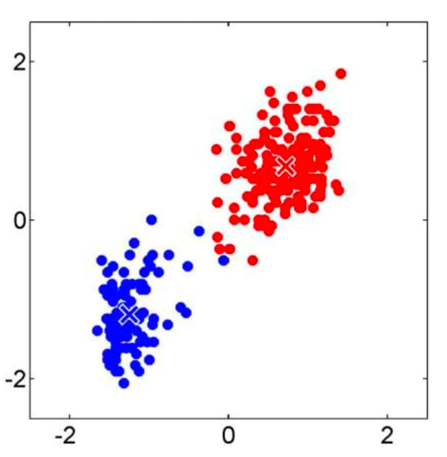
Let’s visualize the algorithm.
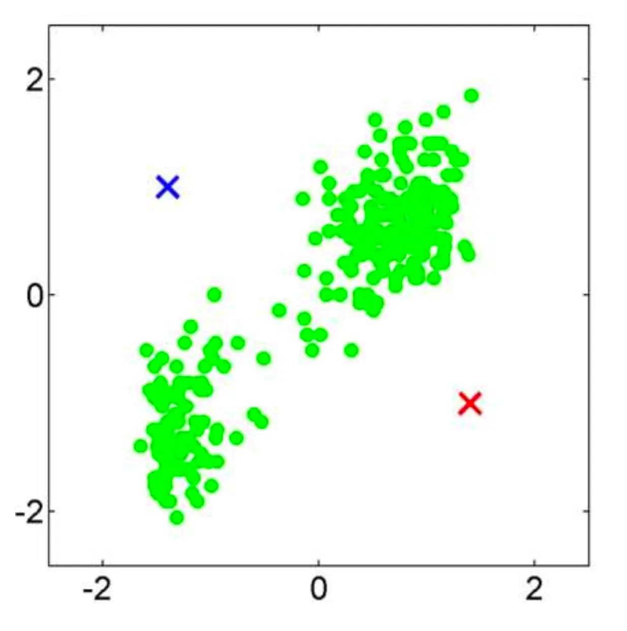
1. Divide the dataset into 2 clusters and assign 2 centroids
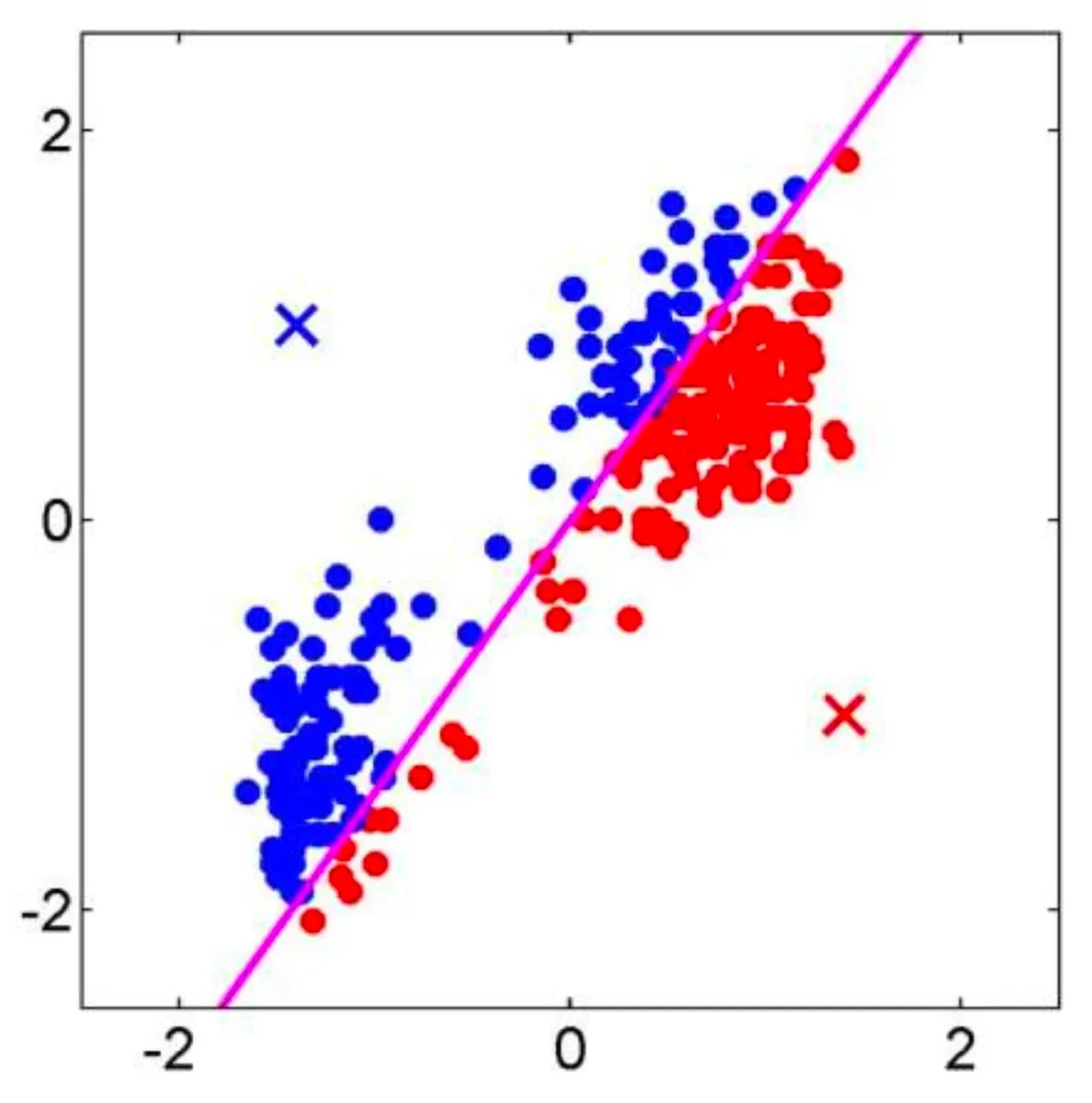
2. Assign each data point to the nearest cluster.
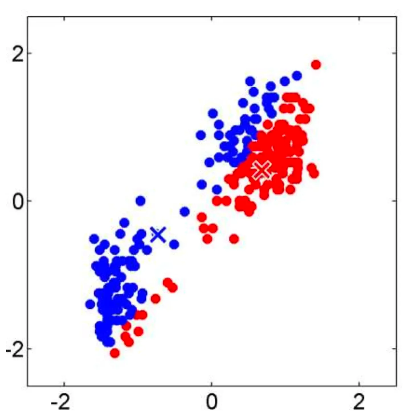
3. Recalculate the centroid of each cluster.
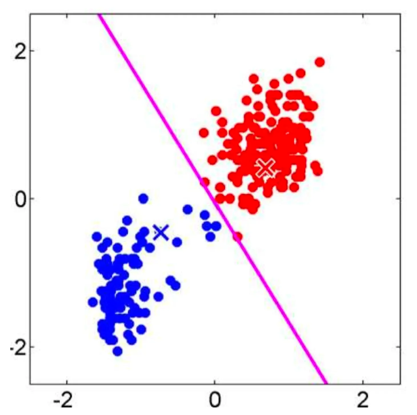
4. Assign each data point to the nearest cluster.
5. Recalculate the centroid of each cluster.
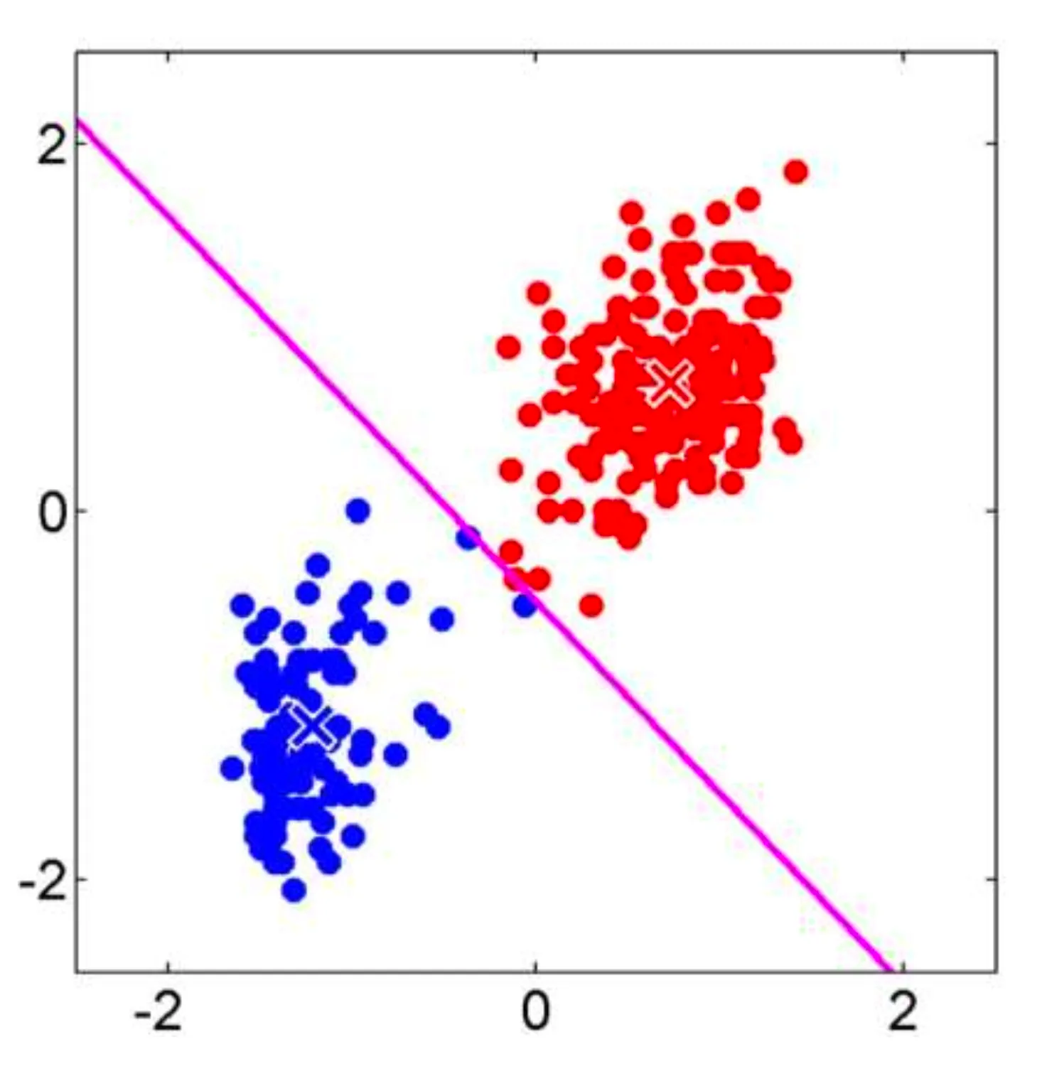
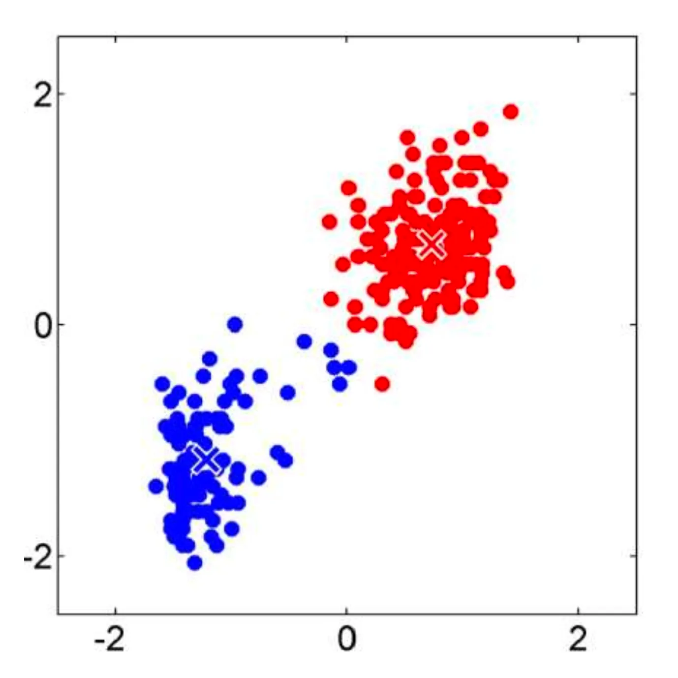
6. Assign each data point to the nearest cluster.
7. Recalculate the centroid of each cluster.
Mathematical Derivation of K-Means
Given the data .
For simplicity, let’s assume , meaning each data point is a 2D coordinate: .
Our aim is to find:
- clusters, each represented by a centroid , where .
- Assignments of each data point to a cluster using an indicator variable:
Let’s define an objective function , which is what we optimize during training to make our model approximate the target function as closely as possible, as
where is the squared Euclidean distance between a data point and its assigned cluster center. The goal is to minimize by optimizing (assignments) and (centroid).
To minimize , we perform two alternating steps:
- Fix , optimize : Assign each data point to the nearest cluster center.
- Fix , optimize : Recalculate cluster centers based on assigned points.
Step 1: Fix , Find
For a single data point , its contribution to is:
To minimize , we assign to the nearest cluster:
This process is repeated for all data points.
Step 2: Fix , Find
Now, we assume data points and are assigned to cluster . We want to find the optimal cluster center that minimizes:
Expanding the squared Euclidean distances:
To minimize , take the derivative and set it to zero. The optimal cluster center is:
or in vector form:
For a general case with more points, the new cluster center is simply the mean of all assigned points:
where is the number of points in the cluster.
K-Means Clustering Using scikit-learn
This is a basic implementation of the K-Means Clustering algorithm using the scikit-learn library:
- Declaration: Begin by importing the
KMeansmodule from the scikit-learn library.from sklearn.cluster import KMeans - Initialization: Specify the number of clusters and create a
KMeansmodel with the number of clusters and arandom_statefor reproducibility.k_cluster = 3 k_mean_model = KMeans(n_clusters=k_cluster, random_state=random_state) - Training: Train the model using the data.
k_mean_model.fit(X)
Linear Regression
Basic Concept of Linear Regression
Linear Regression involves learning a function from a given training set , where , to estimate output values for new observations.
Each observation is represented by an -dimensional vector, , where each dimension represents an attribute or feature.
For example, given the dataset:
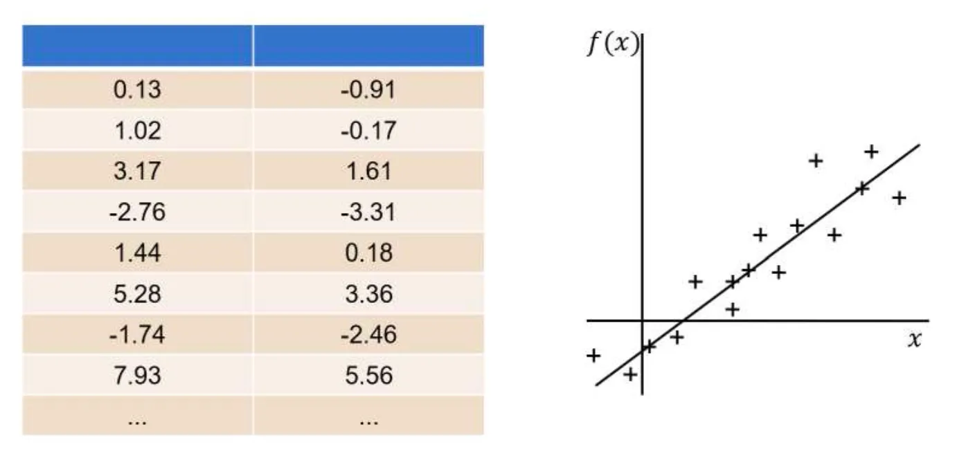
From the dataset, the most optimal linear regression function would be:
Future Value Prediction
In a dataset, each observation consists of multiple input values (features), written as . For each input, there is a true but unknown output value, called .
The machine learning system will try to predict the output value, using a linear function:
Here:
- is the predicted output.
- are weights (which determine how much influence each input feature has).
- are the input features.
Our goal is to make as close as possible to the real value .
Learning a linear regression function means finding the best weights that define the relationship between inputs and outputs.
Once we have these weights, we can use the learned function to predict outputs for new data. If we get a new observation , we use:
This means we multiply each feature by its corresponding weight and sum up the results.
- If we have one input feature , this function represents a straight line.
- If we have two input features , it represents a plane.
- If we have many features , it represents a hyperplane in higher dimensions.
Since there are infinitely many possible linear functions, we need a rule to find the best one. How can we do this?
Learning a Linear Regression Function
Learning a linear regression function, denoted as , involves finding the best linear relationship between input features and an output variable based on a given training dataset. Our aim is to ensure the model generalizes well to new, unseen data.
This involves improving the system performance by minimizing the error, represented as , between the predicted value and the actual value for future inputs .
To measure how well our model is performing, we use a loss function. A popular choice is the empirical loss, also known as the Residual Sum of Squares (RSS), which helps us find the best-fitting line by minimizing the total squared errors.
Loss Function
The basic idea of the loss function is to measure how well our function fits the data by summing up the squared errors. This is called the Residual Sum of Squares (RSS).
We need to find the best function (or equivalently, the best weights that minimizes this error):
Essentially, we are finding the values of that make the squared differences as small as possible.
The best way to find is by setting the derivative of to and solving for .
Linear Regression Using scikit-learn
- Declaration: This involves importing the necessary Linear Regression modules from the scikit-learn library.
from sklearn import linear_model - Initialization: Create a Linear Regression model.
regr = linear_model.LinearRegression() - Training: Train the model using the data.
regr.fit(X_train, y_train) print("[w1, ..., w_n] = ", regr.coef_) print("w0 = ", regr.intercept_) - Prediction: Use the trained Linear Regression model to make predictions by calling the
predict()method on the model object wit the new data as the argument.y_pred = regr.predict(X_test)
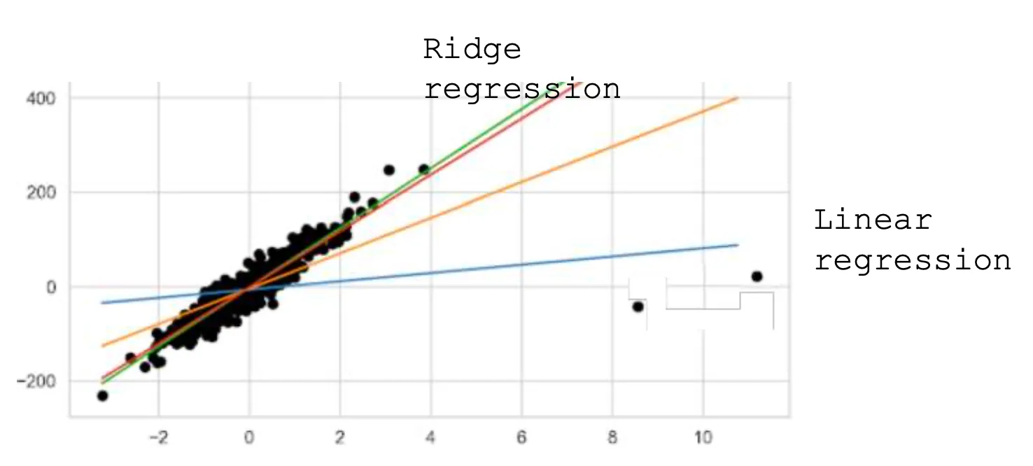
Basic Concept of Ridge Regression
A problem with standard linear regression is that it may not perform well with noisy data because it tries to fit the noise, causing the weights to change drastically.
Ridge Regression is a linear regression technique used to prevent the model's weights from changing drastically, which can occur with noisy data, by adding a penalty. This technique is called regularization and helps the model generalize better to new data.
Instead of just minimizing the usual , we also minimize the sum of squared weights multiplied by a penalty factor . The optimization problem looks like this:
- The first term is the usual , which measures how well the model fits the data.
- The second term is the regularization term, which discourages significant changes in weight values.
- is a tuning parameter that controls how much regularization we apply.
Although Ridge Regression can work with noisy data, it’s a good practice to preprocess the training data beforehand to achieve the best results.
Ridge Regression Using scikit-learn
The only difference of using Ridge Regression in scikit-learn is in the initialization step:
# 'alpha' is the penalty factor
regr_ridge = linear_model.Ridge(alpha = 0.1)
Training the Ridge Regression model:
regr_ridge.fit(X_train, y_train)Support Vector Machine (SVM)
Basic Concepts of SVM
Support Vector Machine (SVM) is a powerful machine learning algorithm used mainly for classification. It tries to find the best possible boundary to separate different classes of data. SVM and its variations include Linear SVM, Soft-margin SVM, and Non-linear SVM.
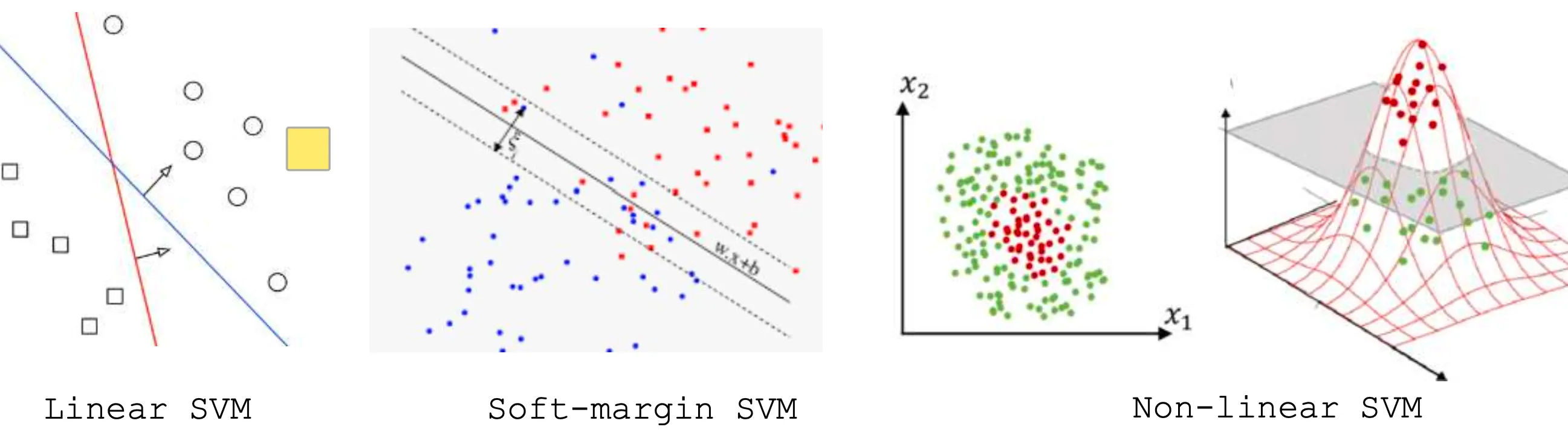
Linear SVM
Linear SVM is a method which works with simple linear separable data that can be divided by a straight line (or a hyperplane in higher dimensions).
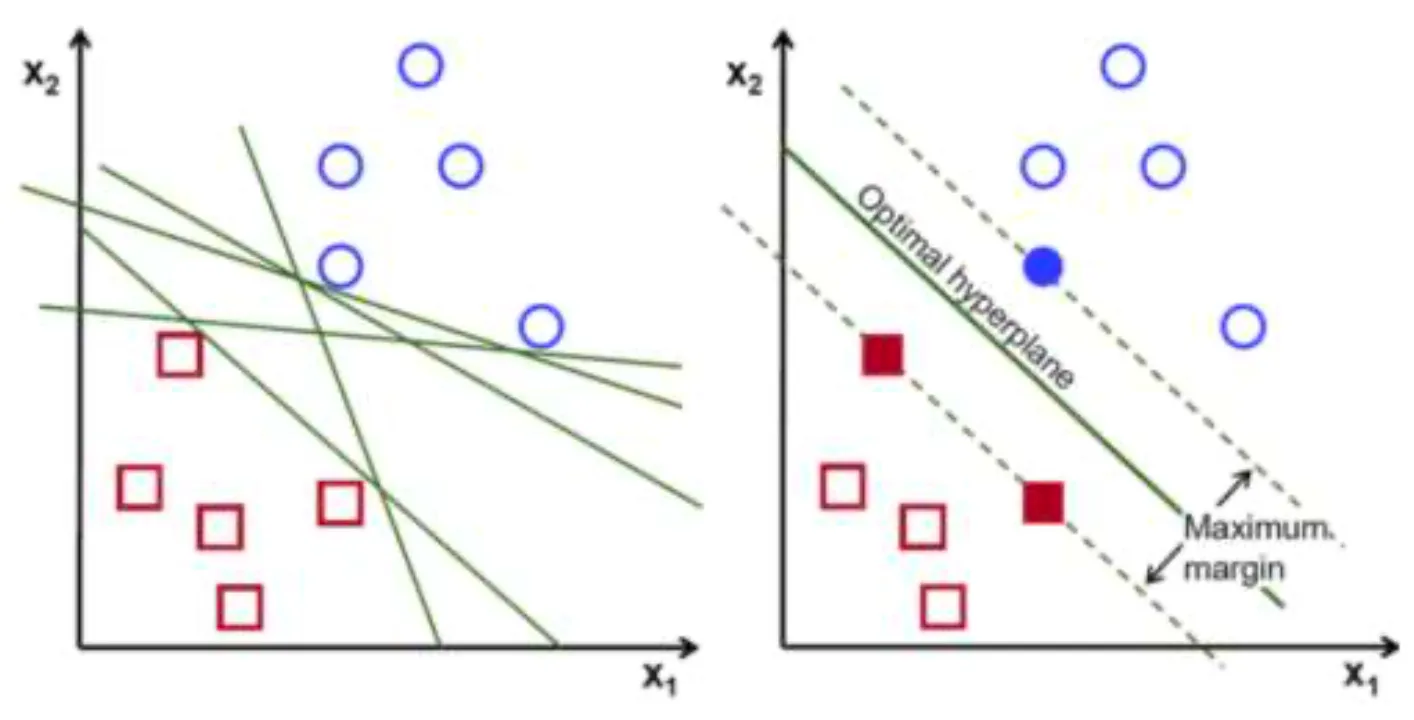
The core idea of Linear SVM is to find a boundary as a line (or hyperplane) that maximizes the distance (margin) between two classes.
Considering we have the dataset , where is an input vector in an -dimensional space with the equivalent output value .
The equation of linear separation function is:
where is the weight vector (determines the direction of the boundary) and is a real number (adjusts the position of the boundary).
The goal is to correctly classify each point, , so that:
There are hyperplanes separating observations of positive () and negative () classes with the equation , and SVM chooses the optimal separating hyperplane with the maximum margin.
Calculating the margin is pretty straightforward.
You first need to select an observation in the positive class and another one in the negative class , where the distance from each observation to the separating hyperplane is the closest.
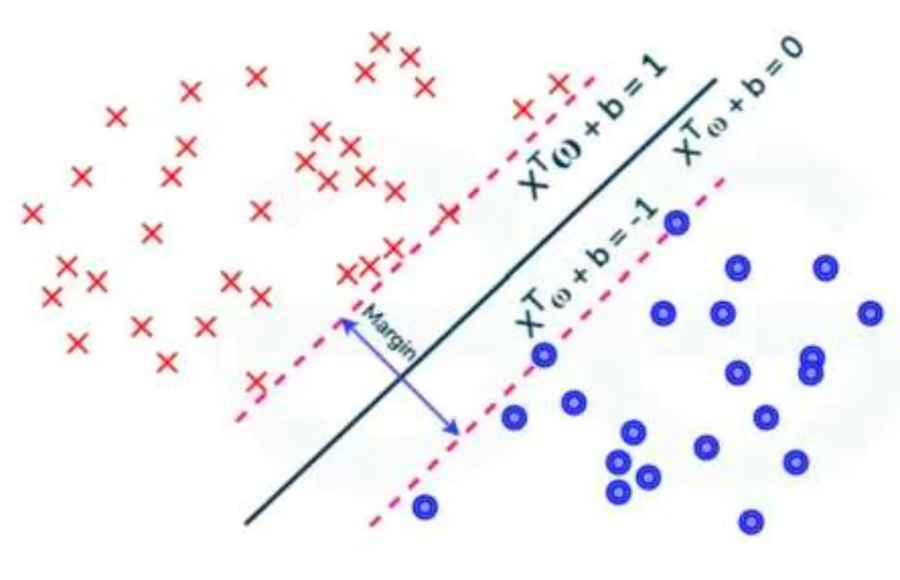
Two parallel support hyperplanes are then defined:
- passes through and is parallel to :
- passes through and is parallel to :
so that .
Now, the margin can be calculated as:
Optimizing Linear SVM
To maximize the margin, we need to minimize . This is where the optimization problem comes in. The objective is to minimize because minimizing is equivalent to maximizing the margin , and the factor of is just for convenience when taking derivatives during optimization.
Finally, SVM solves the following optimization problem to choose the most optimal hyperplane by finding and so that
while subjecting to the constrains of each datapoint with label :
Soft-margin SVM
Sometimes, in real-world data, perfect separation may not be possible (or desirable), especially with data containing noises. Therefore, the Soft-margin SVM method allows some misclassification using slack variables to relax the strict boundary constraints.
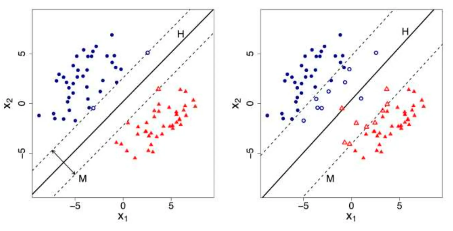
The updated constrains are now:
This means some points can be within the margin or even misclassified, but, at least the errors are minimized!
Non-linear SVM
In many real-world problems, when data cannot be separated by a straight line, Non-linear SVM is used. It transforms the data into a higher-dimensional space, where it becomes linearly separable.
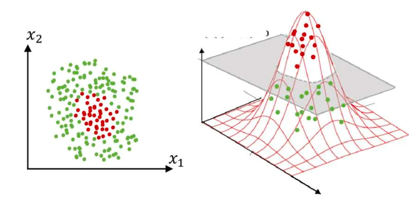
This is done using kernel functions, which map the data to a new space. Some common kernels are:
- Polynomial Kernel
- Gaussian RBF Kernel
- Tanh Kernel
Finally, it applies the same formulas and steps as in linear SVM but in the new transformed space.
Support Vector Machine Using scikit-learn
For Classification Problems
>>> from sklearn import svm
>>> X = [[0, 0], [1, 1]]
>>> y = [0, 1]
>>> clf = svm.SVC()
>>> clf.fit(X, y)
SVC()
For Regression Problems
>>> from sklearn import svm
>>> X = [[0, 0], [2, 2]]
>>> y = [0.5, 2.5]
>>> regr = svm.SVR()
>>> regr.fit(X, y)
SVR()
>>> regr.predict([[1,1]])
array([1.5])
Non-linear SVM
svr_rbf = SVR(kernel = "rbf", C = 100, gamma = 0.1, epsilon = 0.1)
svr_lin = SVR(kernel = "linear", C = 100, gamma = "auto")
svr_poly = SVR(kernel = "poly", C = 100, gamma = "auto", degree = 3, epsilon = 0.1, coef0 = 1)
👏 Thanks for reading!