Basic Sorting Algorithms - DSA #5

In this note, we will explore five elementary sorting algorithms: Bubble Sort, Shaker Sort, Selection Sort, Insertion Sort, and Binary Insertion Sort. We will also take a look at the complexity of each algorithm in detail!

Introduction to Sorting Algorithms

Sorting is something that we’ve seen a lot in real life. A list of names is commonly sorted in alphabetical order, or a list of student grades might be sorted from highest to lowest. In addition, certain searching algorithms, such as Binary Search or Interpolation Search, only works on sorted data. That is the reason why we need sorting algorithms!

Sorting algorithms are methods used to arrange data in a specific order, typically ascending or descending.

They are categorized into comparison-based and non-comparison-based sorting algorithms. Elemental comparison-based sorting algorithms, which we will be discovering in this note, sort elements by comparing them with one another.

Bubble Sort

Basic Concept of Bubble Sort

Bubble Sort is a straightforward comparison-based sorting algorithm that repeatedly steps through a list, compares adjacent elements, and swaps them if they are in the wrong order. This process is repeated until the list is sorted.

The algorithm gets its name because smaller elements “bubble” to the top of the list, while larger elements sink to the bottom.

Bubble Sort Implementation

for (i = 2; i ≤ n; i++)
	for (j = n; j ≥ i; j--)
		// Compare adjacent elements
		if (a[j] < a[j - 1]) 
			a[j] ⇄ a[j - 1]

Performance Analysis of Bubble Sort

The basic operation of this algorithm is the data comparison $a[j] < a[j - 1]$. The complexity analysis of this algorithm has been covered in my previous note, Algorithm Analysis - DSA #2. The total number of comparisons is given by:

Therefore, the time complexity of Bubble Sort is $\Theta(n^2)$.

Since Bubble Sort is an in-place sorting algorithm that requires only a constant amount of additional memory space, its space complexity is $\mathcal{O}(1)$ - constant space.

Shaker Sort

While Bubble Sort is an extremely simple sorting algorithm, it has a few disadvantages. Bubble Sort just compares all adjacent elements without knowing if the array is already sorted! What’s more, the smallest or largest element, when put in the end or the start of the array respectively, moves slowly to their correct position one element at a time, which makes the sorting process super slow! To tackle all of those limitations, Shaker Sort is created, based on the idea of Bubble Sort with rooms for numerous improvements!

An Improvement of Bubble Sort

While Bubble Sort repeatedly traverses the list in a single direction, Shaker Sort improves its efficiency by allowing elements to move in both directions during each pass:

• Move the largest element to the end of the array, similar to Bubble Sort.
• Move the smallest element to the beginning of the array.

• Reduce the size of the array being considered by eliminating elements that are already in their correct positions.
• Repeat until the array is completely sorted.

Shaker Sort Implementation

left = 2; right = n; k = n;

do {
	// Move largest elements to the right
	for (j = right; j ≥ left; j--) {
		if (a[j - 1] > a[j]) {
			a[j - 1] ⇄ a[j]; k = j;
		}
	}
	left = k + 1;
	
	// Move smallest elements to the left
	for (j = left, j ≤ right; j++) {
		if (a[j - 1] > a[j]) {
			a[j - 1] ⇄ a[j]; k = j;
		}
	}
	right = k - 1;
while (left ≤ right);

Performance Analysis of Shaker Sort

Similar to Bubble Sort, Shaker Sort still has a time complexity of $\Theta(n^2)$ in the worse case and a space efficiency of $\mathcal{O}(1)$.

In theory, Shaker Sort should be more efficient than Bubble Sort, as the algorithm reduces the number of comparison operations. However, the number of element exchanges remain unchanged, as we still move an element one-by-one to the correct position in practice. The element exchange operation is actually a compound statement consisting of three assignment operations, and assignment operations take longer than comparison statements (as discussed in Algorithm Analysis - DSA #2).

As a result, there is only a minimal improvement in efficiency comparing to Bubble Sort when Shaker Sort is used in practice.

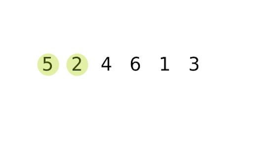
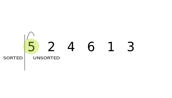
Selection Sort

Different to the previously-mentioned algorithms, Selection Sort moves elements immediately to their final position in the array.

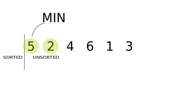
Basic Concept of Selection Sort

The idea behind Selection Sort is pretty simple:

• Scan the entire array to find the smallest element, and swap it with the first element.
• Find the smallest element among the remaining ones, and swap it with the second element.
• Repeat the process until all elements are moved to their correct position.

Selection Sort Implementation

for (i = 1; i < n; i++) {
	minIndex = i; minValue = a[i];
	for (j = i + 1; j ≤ n; j++) {
	// Find the smallest element
		if (a[j] < minValue) {
			minIndex = j;
			minValue = a[j];
		}
	}
	// Move the smallest element
	// to the correct position
	a[minIndex] = a[i];
	a[i] = minValue;
}

Performance Analysis of Selection Sort

In Selection Sort, the basic operation is the comparison $a[j] < \text{minValue}$. The outer loop executes $n - 1$ times, resulting the number of comparisons in the inner loop is $(n - 1) + (n - 2) + … + 1) = \frac{n(n - 1)}{2}$. Therefore, the time complexity of Selection Sort is $\Theta(n^2)$, where $n$ is the number of elements.

Since Selection Sort is also an in-place sorting algorithm, its space complexity is $\mathcal{O}(1)$.

It is also of note that although the number of comparisons performed in Selection Sort is similar to that of Bubble Sort, the number of data movement is significantly reduced, resulting in better performance.

Insertion Sort

Insertion Sort works in a slightly different way. The algorithm is similar to the way one might sort playing cards in their hands, inserting each new card into its proper position among the already sorted cards.

Basic Concept of Insertion Sort

The Selection Sort algorithm works as follows:

• The array is divided into two parts: the left part is always a sorted subarray while the right part is unsorted.

• The first element of the right part, $v$, will be picked up and inserted into the correct position in left part so that the left part is one element larger.

• Repeat the process until the right part is empty.

The question is, how can we insert $v$ into the proper position? The solution is straightforward: check $v$ against all of the elements in the left part.

• If $v$ is smaller than $a[j]$, we will move $a[j]$ to the right one position to create an empty (or free) position. This process stops when the algorithm reaches the first position of the array.

• When the condition is no longer met, the empty position is the correct position for $v$, and $v$ is inserted into that position.

Insertion Sort Implementation

For humans, when we look at an array of numbers, we can easily split the array into the sorted and unsorted part. But how can our computers split the array into two parts?

A simple approach could be scanning the array and find the position to split the array into two halves. However, that is a manual solution and is undesirable. In algorithm design, we always want a system-managed way to do something. Therefore, the most preferable solution would be to split the array so that the left part contains only one element at first.

// At first, the left part 
// contains only one element		
for (i = 2; i ≤ n; i++) {
	v = a[i];
	j = i - 1;
	// Check 'v' against all
	// elements in the left part. 
	while (j > 0 && a[j] > v) {
		a[j + 1] = a[j];
		j--;
	}
	// Insert 'v' into its
	// correct position.
	a[j + 1] = v;
}

Performance Analysis of Insertion Sort

In Insertion Sort, the basic operation is the comparison $a[j] > v$. The outer loop executes $n - 1$ times, resulting the number of comparisons in the inner loop is $(n - 1) + (n - 2) + … + 1) = \frac{n(n - 1)}{2}$ if the list is in reverse order. Thus, the worst-case time complexity of Insertion Sort is $\Theta(n^2)$:

This is also the case with the average-case complexity, however the calculations might be a little bit tricky.

In the best case, when the list is already sorted, the complexity would be $\Theta(n)$ as the condition $a[j] > v$ of the inner loop does not met.

In addition, Insertion Sort requires $\mathcal{O}(1)$ space, making it a space-efficient sorting algorithm.

Binary Insertion Sort

From the above implementation of Insertion Sort, some of you may notice that the operation of determining the correct position of $v$ is actually a Linear Search! A Linear Search has a time complexity of $\Theta(n)$, can we make it even more efficient?

An Improvement of Insertion Sort

The Linear Search in Insertion Sort is actually performed on the left part, which is a sorted subarray! When given a search problem on a sorted array, Binary Search is a good choice! This is the idea of Binary Insertion Sort, which utilizes Binary Search to find the appropriate position to insert $v$.

Binary Insertion Sort Implementation

for (i = 2; i ≤ n; i++) {
	v = a[i];
	left = 1; right = i - 1;
	
	while (left ≤ right) {
		m = (left + right) / 2;
		if (v < a[m]) right = m - 1;
		else left = m + 1;
	}
	
	for (j = i - 1; j ≥ left; j--) {
		a[j + 1] = a[j];
	}
	a[left] = v;
}

Performance Analysis of Binary Insertion Sort

Alright so we’ve already utilized Binary Search in our Insertion Sort algorithm, does it even run any faster?

The algorithm should be more efficient, at least in theory, as it reduces the number of comparison operations performed. However, it does not reduce the number of data movements, and as mentioned above, assignment operations is more costly in terms of time complexity compared to comparisons.

Even though we find the position efficiently using Binary Search, we still need to shift elements to make space for the new element. In the worst case, we need to shift all elements in the left part, which takes $\Theta(n)$ time. Thus, the overall worst-case complexity is:

The space efficiency; however, remained constant at $\mathcal{O}(1)$.

👏 Thanks for reading!