
In this note, I'll guide you through the concepts of machine learning and fundamental types of machine learning problems. I'll also introduce some strategies in designing and evaluating machine learning systems, as well as discussing several insights on data preprocessing!
What is Machine Learning?
Basic Concept of Machine Learning
Machine learning (ML) is a subfield of artificial intelligence that focuses on enabling computer systems to mimic the way that humans learn to perform tasks autonomously, and to improve their performance automatically through experience.
Instead of being explicitly programmed for every possible situation, machine learning systems learn from a large amount of data to make predictions or decisions.

The central question of machine learning is:
How can we build computer systems that automatically improve with experience, and what are the fundamental laws that govern all learning processes? (Mitchell, 2006)
As it goes, a computer with learning capabilities is one that can enhance its performance (P) through a specific task (T) by leveraging its experience (E). Therefore, machine learning revolves around a few fundamental concepts:
- Task (T): This is a specific job or assignment that the machine learning system are designed to perform. This could be anything from predicting house prices to identifying spam emails.
- Performance (P): How well the machine learning system can perform the task. This is measured through a specific metric relevant to the task, such as the number of correctly classified spam emails or the difference between the predicted and actual house prices.


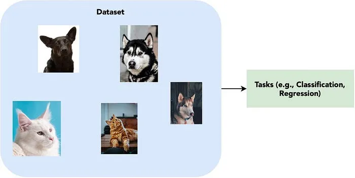
- Experience (E): The data that the system learns from. This is usually a training dataset containing examples with attributes and labels. For example, a collection of emails labeled as spam or not spam, or a dataset of houses with features like size and location, along with their corresponding prices.
In real life, we sometimes prefer reading spam emails over non-spam emails. How can we enhance the performance (P) of the machine learning system to correctly classify emails without losing a single non-spam email? We must consider the experience (E) - the datasets used to train the model.
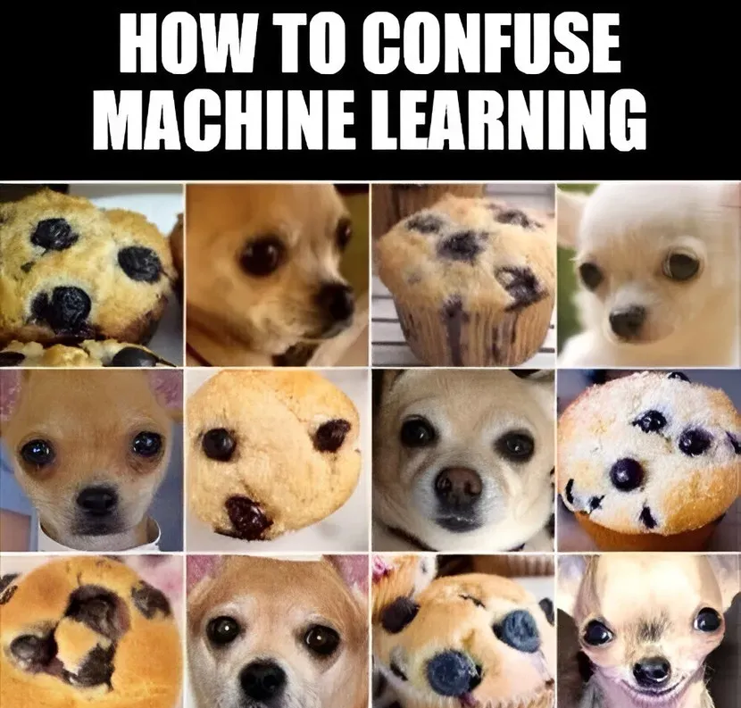
The datasets used to train the machine learning model may contain errors or noises due to the fact that they are usually labeled by a human called a labeler. The labeler's task is to read and classify the dataset for training, such as labeling spam/not spam emails or marking the segments or bounding boxes containing dogs in pictures of dogs, which are often repetitive and can lead to mistakes.
Furthermore, the dataset may not cover all possible cases. For example, if the dataset only includes certain types of spam emails, and the model is trained on that dataset, it may not be able to classify other types of emails correctly. Therefore, it is crucial to ensure that the dataset is generalized to accurately predict future input data.

Core Idea of Machine Learning
Essentially, a machine learning model learns a mapping function, often denoted as , that best maps inputs to predictions . Think of as the input data, and as the model's output.
For example, in a house price prediction task, the machine learning model learns from a training dataset of houses with features (size, location, etc.) and their corresponding prices. The goal is to learn the function that maps house features to prices. Once learned, this function can predict the price of a new house based on its features.
Types of Machine Learning Problems
There are several main types of machine learning problems, each with its approach to learning.
Before getting into these problems, we should know the basic concept of an observation. In machine learning, an observation refers to a single data point in a dataset which consists of several features and, most of the time, a target label.
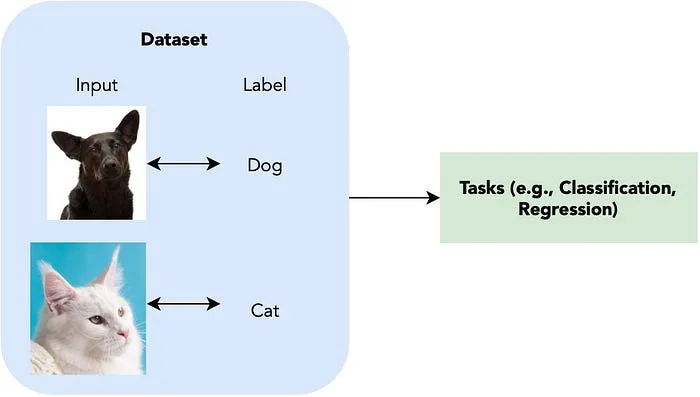
Supervised Learning
Supervised learning involves learning a function from a labeled training set.
The training set consists of paired inputs and outputs , where represents the observations of in the past, and corresponds to the label, response, or output equivalent to .
Once is learned, it can be used to predict the output for a new, unseen input : . This is the stage where the model applies its learned knowledge to make predictions on new data.
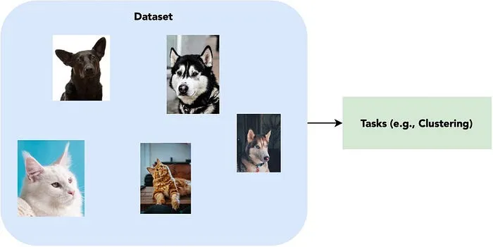
Unsupervised Learning
Unsupervised learning involves learning a function from a given unlabeled training set .
With unsupervised learning, algorithms discover patterns without prior knowledge and focus on identifying the relationships among data points in order to group them together.
Grouping these data points actually provide numerous information, especially in a recommendation system of social media, where these platforms group users based on their activities and present relevant contents to each group without explicitly knowing the interests of each user.
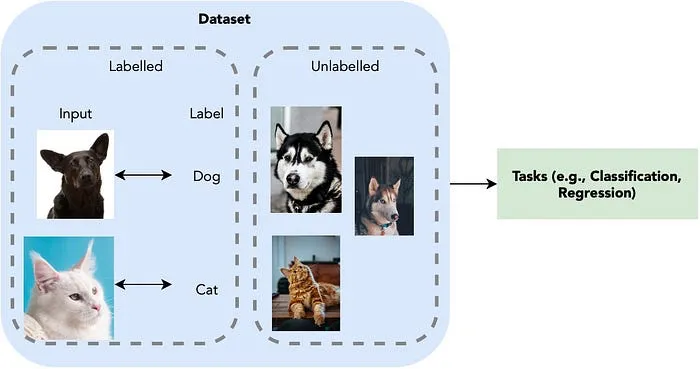
Semi-supervised Learning
Semi-supervised learning uses both labeled and unlabeled data during the learning process. This approach is especially useful when labeled data is limited and unlabeled data is abundant. By incorporating unlabeled data, semi-supervised learning aims to improve model accuracy compared to relying solely on limited labeled data.
In fact, semi-supervised learning is actually pretty interesting. Let's revisit the house prices prediction example once more. By using a classification algorithm, we can categorize houses in the datasets into groups exhibiting similarities. Subsequently, we pre-label these groups, for instance, a group of houses priced around $100,000. These pre-labels are known as pseudo labels. The model is then trained using this dataset. In the future, when it encounters houses with similar characteristics, it will temporarily predict prices of approximately $100,000!
Self-supervised Learning
Self-supervised learning is a technique that leverages vast and diverse unlabeled data sources, where the model still tries to solve traditional supervised-learning problems. This approach contrasts with traditional unsupervised learning, which focuses on relationships between data points rather than understanding individual data point properties and often operates on smaller, specific datasets.
Recent breakthrough in machine learning utilizes this technique, mainly to train foundational (or multimodal) models to accomplish a wide range of tasks. Self-supervised learning, combining with some prompting techniques such as chain-of-thought, can produce “reasoning” models just like the o1 models from OpenAI.
In machine learning, we have “golden labels”, which are manually curated by experts and provide a higher level of certainty in their accuracy. When we refer to the pseudo labels mentioned above, we actually call them “silver labels”, which are not guaranteed to be accurate but still close enough!

Designing Machine Learning Systems
When designing a machine learning system, several key issues must be carefully considered. These includes the data selection, the type of machine learning problem, how to represent the target function, and finally, data splitting.
Data Selection
The training data significantly impacts the effectiveness of the machine learning system. Therefore, selecting the right data is a critical step in designing an effective machine learning system.
The most important consideration of data selection is the ability to obtain the labels for the training data. If we couldn’t get the labeled data, it may not be possible to train a supervised learning model. In addition, the training dataset should be representative of the data that the system will work in the future. If the data isn’t characteristic enough, you won’t get a model with good generalization and it won’t work well on future data.

Identifying the Machine Learning Problem
As mentioned above, the target function is a mapping function that the system learns to predict an output from an input . The nature of determines the type of machine learning problem.
If is a value from a discrete set, like , it's a classification problem; if is a real number, it's a regression problem.
Representation of the Target Function
There are many ways to represent the target function:
- A polynomial function
- A set of rules
- A decision tree
- An artificial neural network
However, the “no-free-lunch theorem” states that no single algorithm can perform best across all domains. If an algorithm performs well on a specific class of problems, its performance will degrade on the remaining problems.
This suggests that with each dataset, we need to determine its properties and which target function representation is best fitted for that dataset.
For example, while Convolutional Neural Networks (CNNs) are great at spotting local features in images, Artificial Neural Networks (ANNs) are better with sequential data like time series, where what came before affects what comes after. It's like trying to use a hammer to screw in a screw; it just doesn't work. So you can't just take a CNN, which is excellent for images, and expect it to be just as awesome for data that's all about sequence.
Data Splitting
When creating a machine learning model, one important step is deciding how to divide the dataset. A common method is to split the dataset into two parts:
- A training set: This is used to teach the machine learning system.
- A test set: This is used to assess the performance of the system after training.
There are some common strategies for splitting data: hold-out, cross-validation, stratified sampling, and bootstrap sampling. For simplicity, only hold-out and cross-validation are discussed in this note.
Hold-out
The hold-out method involves dividing the entire set of examples into two separate, non-overlapping groups: the training set and the test set .
Overall, and usually, . A typical split is and .
To avoid any bias, examples in the test set should not be used during system training. The examples used for training should not also be used to evaluate the system. The data from the test set should provide an unbiased evaluation of the system’s performance.

from sklearn.model_selection import train_test_split

test_size = 0.2
X_train, X_test, y_train, y_test = train_test_split(data_preprocessed,
	data_train.target, test_size=test_size)

print("Training data = ", X_train.shape, y_train.shape)
print("Testing data = ", X_test.shape, y_test.shape)
Training data = (908, 24389) (908,)
Testing data = (227, 24389) (227,)Cross-validation
Cross-validation is a method used to avoid data overlaps between testing sets. With -fold cross-validation, the entire set of examples is divided into non-overlapping subsets (or "folds") of roughly equal size.
During each of iterations, one subset is used as the test set, and the remaining subsets are used as the training set. Then error values (one for each fold) are calculated and averaged to obtain an overall error value. Common choices for are or .
from sklearn.model_selection import ShuffleSplit

test_size = 0.2
cv = ShuffleSplit(n_splits=10, test_size=test_size, random_state=0)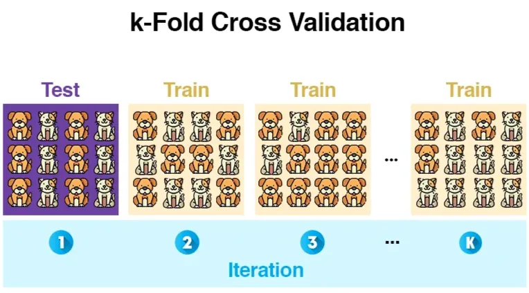
Another approach involves dividing the data into three parts: training, test, and validation sets. The validation set is used to optimize the parameter values in machine learning algorithms.
Parameter Selection
Many machine learning methods use hyperparameters that must be set by the user. For instances, ridge regression uses , and linear SVM uses as hyperparameters. Our machine learning model contains a collection of these parameters.
When designing a machine learning system, selecting the best parameters is crucial for optimal performance. This process, known as model selection, involves choosing the most suitable set of parameters from a learning method. We usually select the parameter that produces the highest performance on the validation set.
Consider we have a limited set that contains potential values for , the dataset for training the model, as well as a measure to assess the performance:
- Initially, the dataset is divided into three disjointed sets: , , and .
- For each value , the algorithm is learned from the training set with the input parameter , and its performance is measured on the validation set to obtain .
- Finally, the with the best is selected, is trained on the set with as the input parameter, and the system’s performance is measured on the test set .

Machine Learning Model Evaluation
Model evaluation is an important aspect of machine learning. It involves using metrics to assess the performance of a trained system. There are several common evaluation metrics: Accuracy, MAE, Precision, Recall, and F1-score.
In Classification Problems
Accuracy
This metric is calculated as the number of correct predictions divided by the total number of predictions.
>>> from sklearn.metrics import accuracy_score
>>> y_pred = [0, 2, 1, 3]
>>> y_true = [0, 1, 2, 3]
>>> accuracy_score(y_true, y_pred)
0.5
>>> accuracy_score(y_true, y_pred, normalize=False)
2.0Confusion Matrix
A confusion matrix provides information on the classes that a classification model is mistaking.
To understand the confusion matrix, it is important to understand True Positives (TP), False Positives (FP), True Negatives (TN), and False Negatives (FN).
For a specific class , the confusion matrix contains the following elements:
- True Positives (): The number of instances of class that are correctly predicted as .
- False Positives (): The number of instances that do not belong to class but are incorrectly predicted as .
- True Negatives (): The number of instances that are not in class that are also correctly predicted as not in class .
- False Negatives (): The number of instances of class that are incorrectly predicted as not belonging to .
For example, in email spam filtering, a TP would be a spam email correctly identified as spam, while a FP would be a non-spam email incorrectly marked as spam.
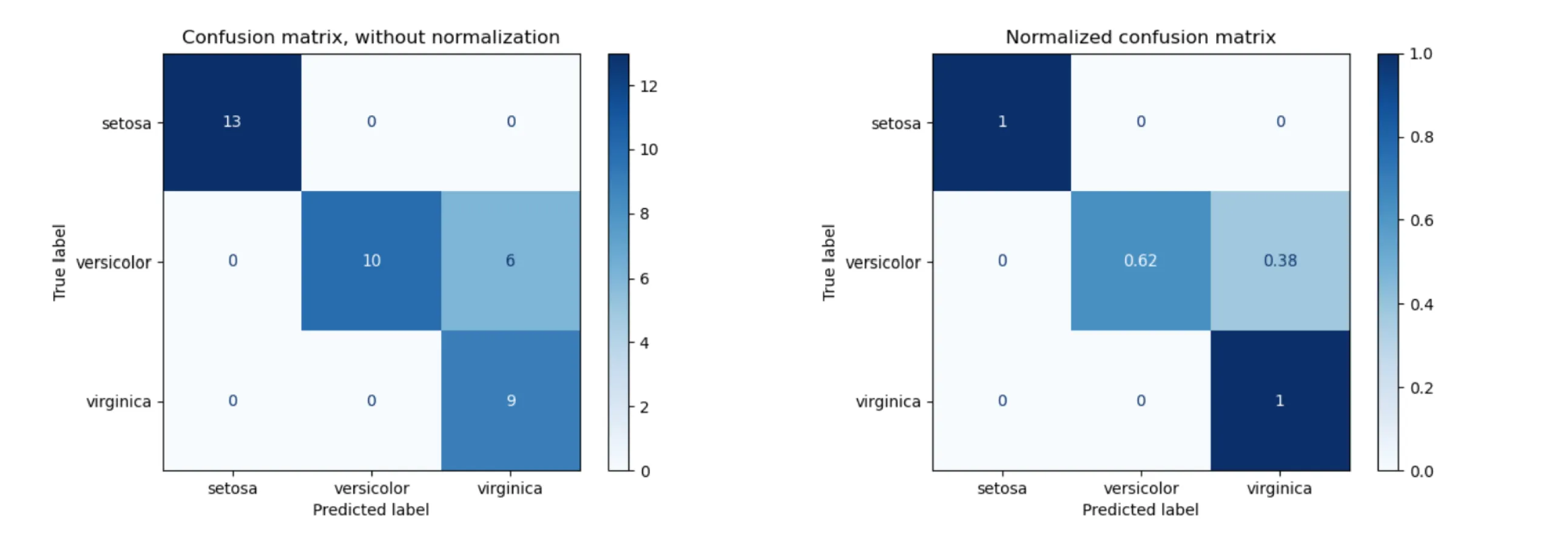
Explanation for the above example confusion matrix
- Left Confusion Matrix (Without Normalization)
- This matrix shows the raw count of correct and incorrect predictions.
- The rows represent actual (true) labels, while the columns represent predicted labels.
- Diagonal elements indicate correct classifications:
- 13 Setosa samples were correctly classified as Setosa.
- 10 Versicolor samples were correctly classified, but 6 were misclassified as Virginica.
- 9 Virginica samples were correctly classified.
- The off-diagonal elements indicate misclassifications:
- 6 Versicolor samples were predicted as Virginica.
- Right Confusion Matrix (Normalized)
- This version normalizes the values row-wise (per class), converting counts into proportions.
- The sum of each row is 1, indicating how often each true class is predicted correctly or misclassified.
- Setosa is classified correctly 100% of the time.
- Versicolor is correctly classified 62% of the time, but 38% are misclassified as Virginica.
- Virginica is correctly classified 100% of the time.
>>> from sklearn.metrics import confusion_matrix
>>> y_true = [2, 0, 2, 2, 0, 1] # Actual class labels
>>> y_pred = [0, 0, 2, 2, 0, 2] # Predicted class labels
>>> confusion_matrix(y_true, y_pred) # Classes in this case are {0, 1, 2}
array([[2, 0, 0],  # Class 0
      [0, 0, 1],  # Class 1
[1, 0, 2]]) # Class 2Explanation for the above code
The confusion matrix format follows:
From the output:
| True Label → Predicted Label ↓ | Class 0 (Actual) | Class 1 (Actual) | Class 2 (Actual) |
| Class 0 (Predicted) | 2 (correct) | 0 (misclassified) | 1 (misclassified) |
| Class 1 (Predicted) | 0 (misclassified) | 0 (correct) | 0 (misclassified) |
| Class 2 (Predicted) | 0 (misclassified) | 1 (misclassified) | 2 (correct) |
- Class 0: 2 samples correctly predicted (
[0,0]entry). - Class 1: 1 sample was supposed to be class 1 but was misclassified as class 2 (
[1,2]entry). - Class 2: 2 samples correctly predicted (
[2,2]entry), but 1 sample was misclassified as class 0 ([2,0]entry).
Key observations:
- Class 0 (Actual): 2 correct predictions, no misclassifications.
- Class 1 (Actual): All samples were misclassified (1 as class 2).
- Class 2 (Actual): 2 correctly classified, but 1 was misclassified as class 0.
Precision and Recall
Precision for class is calculated as the number of correctly classified examples of class divided by the total number of examples classified as .
Recall for class is calculated as the number of correctly classified examples of class divided by the total number of examples belonging to class .
To calculate precision and recall for the entire set of classes , micro-averaging and macro-averaging can be used.
Micro-averaging calculates precision and recall by summing the true positives (TP), false positives (FP), and false negatives (FN) across all classes.
Macro-averaging calculates precision and recall by averaging the precision and recall for each class.
F1-score
This is a harmonic mean of precision and recall.
>>> import numpy as np
>>> from sklearn.metrics import f1_score
>>> y_true = [0, 1, 2, 0, 1, 2]
>>> y_pred = [0, 2, 1, 0, 0, 1]
>>> f1_score(y_true, y_pred, average='macro')
0.26...
>>> f1_score(y_true, y_pred, average='micro')
0.33...In Regression Problems
Mean Absolute Error (MAE)
This is calculated as the average absolute difference between the actual value and the predicted value.
- : The output (predicted value) by the system for example .
- : The actual (true) output value for the example .
>>> from sklearn.metrics import mean_absolute_error
>>> y_true = [3, -0.5, 2, 7]
>>> y_pred = [2.5, 0.0, 2, 8]
>>> mean_absolute_error(y_true, y_pred)
0.5Data Preprocessing
Data preprocessing is a crucial step in machine learning because real-world data is often incomplete, noisy, and inconsistent.
- Incomplete data: The data may be missing attribute values, e.g.,
Occupation=""(missing data). - Noisy data: The data may contain errors, outliers, or noise, e.g.,
Salary="-10"(an error). - Inconsistent data: The data may contain discrepancies in codes or names, e.g.,
Age="42", Birthday="03/07/2010", rating values varies from"1, 2, 3"to"A, B, C", discrepancies between duplicate records, etc.

Data Cleaning
- Filling in missing values: This addresses the issue of incomplete data, where some attribute values are missing. Techniques to handle missing values include:
- Ignoring the tuple with the missing value.
- Manually filling in the missing value - the most preferred technique.
- Assigning a special label or a value outside the range of representation.
- Filling the value with the mean (average) of other values.
- Filling the value with the mean of other samples belonging to the same class.
- Using machine learning models to predict the missing value.
- Reducing noise: This step addresses noisy data by removing errors and outliers. Smoothing techniques, such as binning, clustering, and regression, can be used to reduce noise.
- Resolving inconsistencies: This involves checking and correcting inconsistencies in the data, such as differences in codes or names.
Data Transformation
Data transformation is a data preprocessing method that involves converting the entire set of values of a given attribute to a new set of replacement values. It enhances data quality and model performance.
Methods for data transformation include:
- Smoothing: Reducing noise using techniques like binning, clustering, and regression.
- Normalization: Scaling attribute data values to a smaller range, such as through min-max normalization, z-score normalization, or normalization by decimal scaling.
- Min-max normalization to :
Example: The income range from to is normalized to . In that case, is transformed as .
- Z-score normalization (: mean, : standard deviation):
Example: Given , , then .
- Normalization by power of 10:
where is the smallest integer such that .
- Min-max normalization to :
- Discretization: Converting continuous attributes into discrete intervals.
👏 Thanks for reading!