
In this note, we will explore three searching algorithms: Linear Search, Binary Search, and Interpolation Search. Additionally, we will analyze the performance of each algorithm in detail!
Introduction to Searching Algorithms
A searching algorithm is a method for finding a specific element within a data collection.
In this note, we’ll be analyzing three algorithms for searching the contents of an array: Linear Search, Binary Search, and Interpolation Search.
For simplicity, we’ll assume the data is stored in an array of positive integers and may or may not contain duplicate values.
Linear Search
Basic Concept of Linear Search
Linear Search (also known as sequential search) is the simplest form of searching:
- It starts at the beginning of the array.
- Each element is compared in turn with the target search key.
- The process stops when a match is found or when the end of the array is reached, indicating that the target is not present.
Linear Search Implementation
Here’s the pseudo-code of Linear Search:
i = 1;
while (i ≤ n && a[i] != k) i++;
	// Continue stepping through the array
	// by incrementing 'i' if when a match
	// hasn't been found or it's not at the
	// end of the array.
return (i ≤ n);
An alternative version which uses a sentinel to simplify the loop control:
a[n + 1] = k; // A sentinel
i = 1;
while (a[i] != k) i++;
return (i ≤ k)
Performance Analysis of Linear Search
As discussed in my previous note, Algorithm Analysis - DSA #2, we all agree that is the basic operation of this algorithm. The reason for this is pretty obvious: it is located in the inner-most loop, and it is related to the data that needs to be processed which is the array .
I’ve already included a detail analysis of the complexity of the Linear Search algorithm in that note as well. Basically, the best-case time complexity of linear search is , the average case is , while the worse case is .
As a result, the Big notation of Linear Search is — linear time complexity.
In addition, Linear Search has a space complexity of — constant space. It uses no additional data structures to find the search key!
| Best-case Complexity | |
| Average-case Complexity | |
| Worst-case Complexity | |
| Space Complexity |
The Linear Search is very intuitive and easy to implement. However, its major drawback is inefficiency—especially with large arrays, as in the worst case it requires scanning every element. 😞
Binary Search
Basic Concept of Binary Search
Binary Search is a more efficient algorithm, especially for large arrays, but it comes with a key requirement: the array must be sorted.
The idea is to repeatedly divide the array in half:
- Begin by comparing the search key with the middle element.
- If the key equals the middle element, the search is successful.
- If the key is less than the middle element, then the target (if it exists) must lie in the left half of the array.
- Conversely, if the key is greater, the search continues in the right half.
This halving process continues until the target is found or the subarray reduces to zero.
By the way, here’s a fun story, adapted from “The Tortoise and the Hare”, to demonstrate the importance of pre-sorting the array in Binary Search:

The Tortoise and the Hare: The Search Algorithm Race
In a competition to find an element in an array filled with multiple values, the Hare was proud of its high efficiency, using Binary Search with a time complexity of . It looked down on the Tortoise, who relied on Linear Search with a complexity of .
As soon as the race started, the Hare immediately applied the divide and conquer technique, swiftly leaping over half of the array without examining each element individually. Just as it thought victory was near, the Hare suddenly realized: "My array isn’t sorted!"
Panicked, the Hare had to rush back to the starting line to sort the data first.
Meanwhile, the Tortoise, with patience and determination, steadily moved forward step by step, examining each value in the array without skipping any information. Although it moved slowly, every step brought it closer to the goal with certainty.
In the end, while the Hare was still struggling to organize its data to fit its algorithm, the Tortoise successfully reached the target by carefully scanning each element one by one, without requiring any prior sorting.
Thus, in cases where data is not well-organized, a ”slow but steady” method like Linear Search can sometimes outperform a ”fast but risky” approach like Binary Search. The lesson learned from this story is that choosing the right algorithm depends on the specific conditions of the data, and we should never underestimate the simplicity and reliability of an alternative method, even if its time complexity appears less efficient.
Binary Search Implementation
left = 1, right = n;
// left: the left-most index of the subarray
// right: the right-most index of the subarray

while (left ≤ right) {
	middle = (left + right) / 2;
	if (a[middle] == k)
		return true;
	else
		if (k < a[middle])
			right = middle - 1;
			// element will be found in
			// the left half of the array
		else
			left = middle + 1;
			// element will be found in
			// the right half of the array
}
return false
Performance Analysis of Binary Search
Let be the size of our input data. In each iteration, Binary Search halves the search space:
After the final step, the search space is reduced to a single element, meaning:
Rearranging and solving for :
Thus, the worst-case time complexity of Binary Search is .
is also the average case, since the number of iterations required to find an element is still proportional to . Since each step reduces the search space exponentially, even randomly distributed elements are found within comparisons.
As for the best case, if the target element is found in the first comparison (i.e., it happens to be the middle element), Binary Search completes in one step. Mathematically, this means .
Binary Search requires no extra data structures; therefore, the space complexity of Binary Search is – constant space.
| Best-case Complexity | |
| Average-case Complexity | |
| Worst-case Complexity | |
| Space Complexity |
Interpolation Search
As humans, when we search for something, we naturally focus on the area where it is most likely to be found. For example, if we are looking for the word “structure” in a dictionary, we would typically start searching near the end, where words beginning with “S” are located.
This intuitive approach to searching is highly effective, and if we apply the same principle in computing, we can develop an efficient search algorithm. This idea forms the basis of Interpolation Search.
Basic Concept of Interpolation Search
Interpolation Search is an algorithm designed to efficiently locate a specific value within a sorted array of uniformly distributed elements. Unlike Binary Search, which consistently examines the middle element of the current search range, Interpolation Search estimates the probable position of the target value based on its relationship to the end of the array:
- Define the initial search boundaries with set to the first index and set to the last index of the array.
- Calculate the estimated position () of the target value () using the formula:
This formula assumes a linear distribution of values and predicts where the target might be located within the current bounds.
- Compare the search key () with the predicted position:
- If equals the , the search is successful.
- If is less than the , adjust the boundary to .
- If is greater than the , adjust the boundary to .
- Repeat the estimation and comparison steps until the is found or the search range is exhausted.
The reason behind that formula? Let’s plot the elements of our array and its indices onto a Cartesian plane.
The algorithm predicts the likely index () using proportionality between the value range and the index range.
The above formula is derived from the slope of the line connecting the points , .
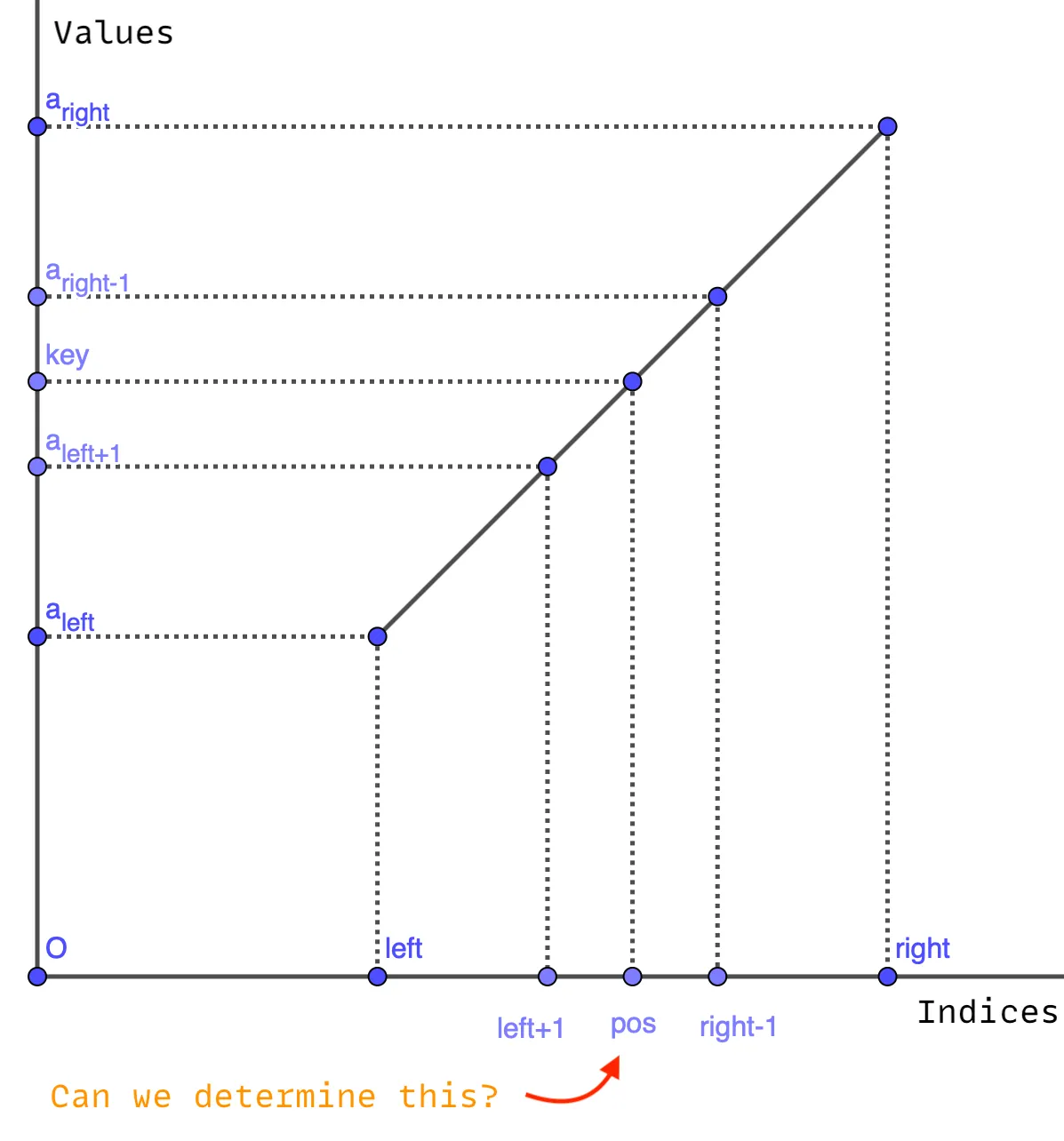
We’re seeing a line here because we assume that the array consists of uniformly (or approximately linearly) distributed values. In reality, it should be a zigzag rather than a line, as the values can be skewed or clustered. In that case, the algorithm’s efficiency diminishes.
Interpolation Search Implementation
Here’s the pseudo-code implementation of the above concept:
left = 1, right = n;
while (left ≤ right && x ≥ a[left] && x ≤ a[right]) {
	pos = (((x - a[left]) * (right - left)) /
		(a[right] - a[left])) + left;
	if (a[pos] == x) return true;
	else if (a[pos] < x) left = middle + 1;
	else if (a[pos] > x) right = middle - 1;
}
return false;
Performance Analysis of Interpolation Search
In Binary Search, the search space shrinks by a factor of 2 in each step, leading to a time complexity of .
However, in Interpolation Search, the reduction depends on the distribution of the data. If the data is uniformly distributed, each step reduces the search space proportionally, not necessarily by half.
Initial:       [● ● ● ● ● ● ● ● ● ● ● ● ● ● ● ●]  (n elements)
Step 1:        [● ● ● ● ● ● ●]-----------------   (≈ n^(1/2))
Step 2:        [● ● ●]-------------------------   (≈ n^(1/4))
Step 3:        [●]-----------------------------   (≈ n^(1/8))
Final Step:    Target found!
Calculating the average-case time complexity of Interpolation Search is a little bit tricky and we’re gonna leave it to the professionals, instead, we just care about the complexity itself, which is .
Interpolation search performs poorly when the data is skewed or non-uniformly distributed (e.g., exponential, clustered values), the interpolation formula estimates wrong positions repeatedly, leading to inefficient jumps, or the target is not in the array, requiring a full scan. In such cases, the search does not effectively reduce the search space, leading to a worst-case complexity of .
If the target element is exactly at the estimated position on the first attempt, the search completes in one step, making the time complexity .
Interpolation Search requires no extra data structures; therefore, the space complexity of Interpolation Search is – constant space.
| Best-case Complexity | |
| Average-case Complexity | |
| Worst-case Complexity | |
| Space Complexity |
In reality, Interpolation Search is too good to be practical, and Binary Search is good enough for most cases.
| Algorithm | Best Case | Average Case | Worst Case |
| Binary Search | |||
| Interpolation Search |
👏 Thanks for reading!